Indiana Jones and the Seismic Anomaly: The Potential of Seismic Methods in Archaeology

Introduction

The painstaking and time-consuming nature of archaeological excavation makes it important to locate potential targets as accurately as possible before digging. Field archaeologists mostly rely on their experience, knowledge and intuition to stake out the most fruitful excavation locations at a site, unless, like Indiana Jones, they have a cryptic old treasure map. Efforts are now being made to assist the archaeologist’s intuition with the introduction of geophysical survey techniques aimed at locating shallow anomalous zones that may correspond to buried features of archaeological interest. These may include void spaces (tunnels or chambers), ‘hard’ zones (stone structures) or disturbed zones (burials, etc.). Potentially detectable archaeological targets must differ from the background earth materials in one or more physical properties: density, elastic wave velocity, conductivity or magnetic susceptibility. They may interrupt existing layer boundaries or they may themselves have distinct boundaries. An acceptable survey method should be able to detect such targets and show their location and size with some accuracy and it must not generate ‘false positive’ anomalies, which might lead to wasted excavation effort. In addition, a geophysical technique should be fast and cheap and should itself cause no disruption of the earth or its contents.

Methods like gravity, magnetic and electrical conductivity surveys are cheap and easy, but they seldom resolve targets precisely enough for archaeological purposes. One technology which has shown promise, however, is ground penetrating radar (GPR). When soil and groundwater conditions are suitable, a GPR survey is one of the more reliable detectors of buried void spaces and zones of disturbed layering in the near surface. Soil conditions, however, are the Achilles’ heel of GPR, since radar only works well in relatively resistive media. The penetration depth of electromagnetic energy into the ground is inversely proportional to the soil conductivity and to the signal frequency, and many areas with conductive groundwater and/or significant clay mineral content support very little radar penetration. In addition, while GPR can usually accurately locate an anomaly laterally, depth determination can be problematic.

A seismic survey, however, can be conducted successfully almost anywhere; and proper imaging and analysis of the data can localize a target both laterally and vertically. Shallow seismic techniques are still relatively new, however, and few efforts have yet been made to apply seismic techniques specifically to the location of archaeological targets. In the following, we discuss some possible approaches for using seismic methods for archaeology and show some early efforts at CREWES to use seismology to assist archaeologists working at two Mayan archaeological sites in Belize.

Shallow Seismic Techniques

Conventional seismic survey methods, developed to a high degree of sophistication over the past several decades, are not suited to exploring the very near surface because of their large scale. They are intended to image regions of the subsurface hundreds or thousands of metres deep, so conventional seismic acquisition systems use very energetic sources and large numbers of geophones widely distributed over the earth’s surface. A field crew consisting of several specialists and a number of casual labourers is required to deploy and operate such systems. This makes them far too expensive and unwieldy to use for small-scale surveys.

Adaptation of seismic methods for imaging very shallow objectives is a relatively recent development (Steeples et al., 1985, 1986, 1988; Miller et al., 1988). Shallow surveys are usually performed with portable seismic recorders having a limited number of channels (60 is a typical number), single geophones and relatively weak (and cheap) surface sources (don’t even mention dynamite to an archaeologist!). Surveys of this scale can be performed rapidly by as few as two people, so that acquisition costs and time are similar to those for a GPR survey.

A consequence of the limited number of channels used for shallow seismic recording is often either a limited range of source-receiver offsets or low data redundancy (fold). The use of a surface source creates its own special problems, since such sources readily excite large amplitude surface, refracted and guided wave modes. These linear modes may themselves be useful for some types of imaging (such as tomography) but they must be greatly attenuated in order to image shallow reflections. Pre-stack noise attenuation is usually necessary, since the fold of shallow surveys is often insufficient to attenuate the coherent noise by stacking alone. The very shallowest reflections may appear on only the two or three traces nearest the source without exceeding the critical angle. Any associated refraction energy must be removed as completely as possible from such offset-limited events prior to analyzing NMO velocities or stacking, or the resulting stacked ‘reflection’ may actually consist mostly of refraction energy.

Focusing on Archaeology

To determine how useful seismic techniques can be for archaeological purposes, we must first consider what physical characteristics of archaeological features will make them seismically detectable. Generally, targets of interest for excavation lie in the uppermost few metres of the earth. Exceptions, like deep tunnels or chambers, will be ignored here. A common characteristic of many archaeological sites is that interesting features are located in the soil/rubble zone above the first competent bedrock layer (e.g., old structures) or else involve some disruption of the bedrock surface itself (e.g., burial chambers). An archaeological target of either variety should be seismically detectable if it differs significantly in either velocity or density from its surroundings. The shape, size and orientation of a target also influence its seismic detectability, depending upon the particular kind of seismic observation employed.

Archaeological seismic surveys will almost always have sources and receivers located only on the earth’s surface; so reflection seismic methods, which rely primarily on vertically propagating seismic energy, will image mostly horizontal boundaries between regions of different velocity/density. Hence, reflection imaging will be most suitable for finding targets with horizontally oriented surfaces or for finding disruptions of known horizontal boundaries like the bedrock surface or layers within the weathered zone above the bedrock. Vertical boundaries will not be readily seen on reflection images. A further requirement for successful reflection imaging is that a reflecting interface represents a relatively abrupt change in acoustic properties.

Restricting sources and receivers to the surface also means that transmission seismic methods (tomography, for example), which are insensitive to abrupt boundaries but respond to distributed changes in velocity/density, are constrained to use mostly horizontally propagating seismic energy to detect local changes in velocity/density. Targets with vertical boundaries will be detectable by these methods, but only if they have significant lateral thickness and/or velocity difference with respect to the background. The target boundaries themselves need not be abrupt, however, for tomographic imaging.

Ideally, we would like to detect an anomaly using both a vertically illuminated reflection image and a horizontally illuminated tomographic image. Most often, however, we expect the situation where an anomaly will only appear on one image or the other. In this case, confirmation of the anomaly could come from coincident anomalies on images from one or more other seismic lines which tie the original line.

A Useful Field Technique

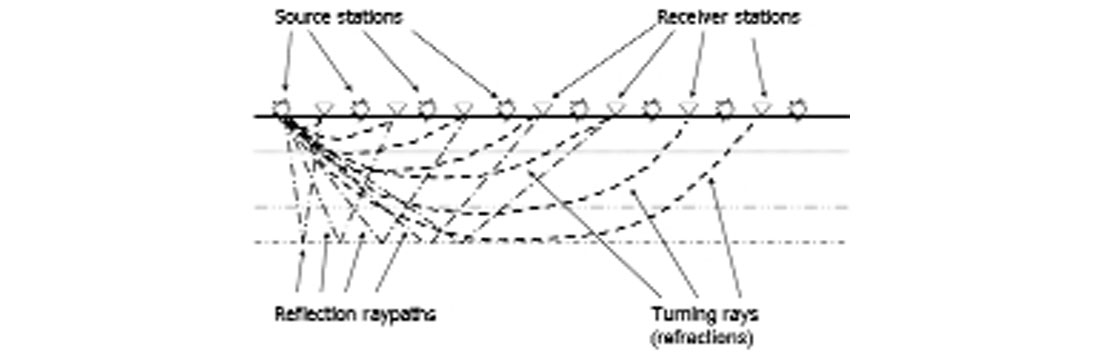
Over the course of three field experiments a simple survey technique has emerged: a typical archaeological survey is only a few tens of metres in length, so a geophone spread can often be deployed and remain fixed for the entire survey. A moving source, as shown in Figure 1, can then ‘shoot through the spread’. Single geophones are used at the stations and simple surface sources (sledgehammer blows) are used. The geometry shown in Figure 1, with source points between the receiver positions, is suited to both reflection imaging and refraction tomography. For reflection imaging, source and receiver gathers have the same spatial sampling, which is useful for linear noise attenuation. Placing the source points between the receivers tends to decouple the source and receiver statics and reduces the chance of overdriving geophones close to the source. For turning ray tomography, the geometry of Figure 1 leads to a reasonably uniform density of raypaths in most velocity models, making the corresponding images relatively robust.

For the geometry depicted in Figure 1, reflections become more robust as depth approaches a half spread length, due to increasing fold. On the other hand, the turning ray tomographic model mainly applies to the region of the earth less than a half spread length in depth. As a general rule, refraction tomographic anomalies are more believable in the shallow part of the earth and reflection anomalies become more believable with increasing depth (up to perhaps a spread length).

Examples

To demonstrate the possibilities for using seismic methods in archaeological assessment, we next show results obtained from three different seismic surveys conducted at two Mayan temple sites in Belize. None of the work shown is complete, however, nor have any anomalies yet been confirmed by excavation. While very suggestive, all examples shown here remain speculative until such time as they are either verified or discredited by digging.

So, where’s the tomb?

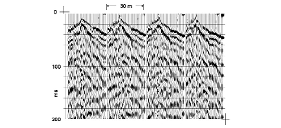
Our first experimental survey was carried out in 2000 at the Chan Chich archaeological site in Belize, where undiscovered burial sites are considered to be among the possible targets. A set of 10 3-C geophones was planted at 1 m intervals along a 9 metre line on the surface of the ‘plaza’ in the vicinity of a Mayan pyramid. Thirty source points were located along the line from 10.5 metres off the low receiver station to 10.5 metres off the high receiver station in order to give 20 metres of CDP coverage. Multiple blows of a sledgehammer, stacked at each source point, provided the seismic energy for the survey and all three particle motion components were recorded. Figures 2 and 3 show receiver gathers of the vertical and inline horizontal components, respectively. At first glance, both vertical and inline components look the same, and there are no visible reflections on either; the records are dominated by coherent noise.

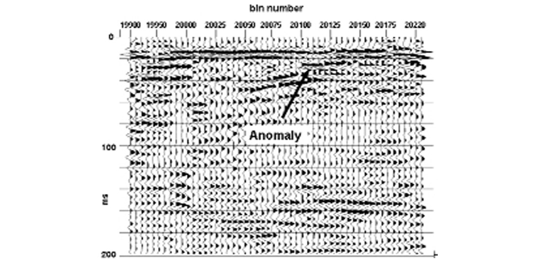
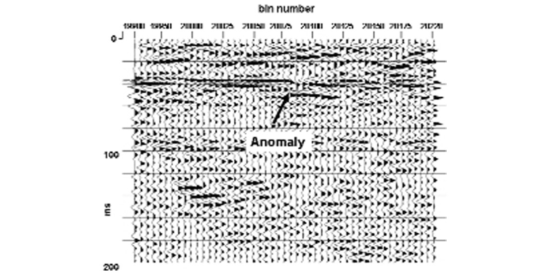
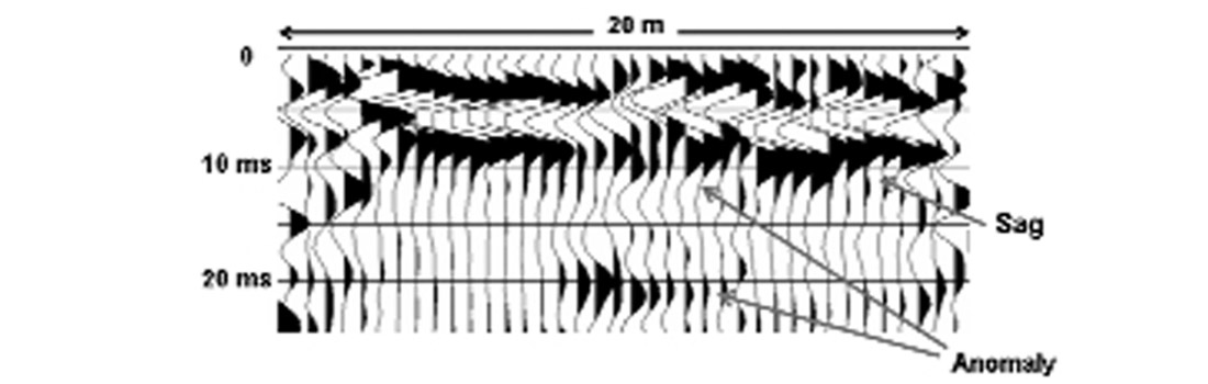
After some intensive processing (Henley, 2001), which includes several contiguous radial trace filter passes to attenuate coherent noise before stack, reflection images were obtained for both compressional (P-P) and converted (P-S) energy. These images are shown in Figures 4 and 5, respectively. Several observations pertain to these images: Firstly, they both show a prominent shallow reflection, probably bedrock, which appears to be interrupted near the centre, with a fragmentary reflection (or diffraction) just beneath it. Secondly, event travel time differences and measured NMO velocities imply a very large ratio of compressional to shear velocity (at least 5:1) for the material above the reflecting interface. Finally, partly as a consequence of the very slow shear velocity, the P-S image in Figure 5 has much greater vertical resolution than the P-P image in Figure 4. Significantly, we found that both the vertical and the inline horizontal component data contained significant contributions from both P-P and P-S modes. It was possible to process either data set to obtain both P-P and P-S images. Distinct anomalies like those in Figures 4 and 5 were seen only on two of the images, however, leading us to regard the anomaly as questionable.

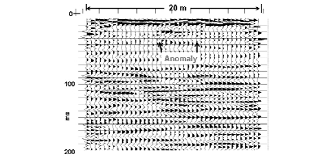
A second survey was conducted at Chan Chich in 2001 over the same profile as the 2000 survey. In this instance a spread of 20 3-C phones spaced at 1 metre intervals along a 19 metre line was used, with 21 source points between the stations and 0.5 metre off each end of the spread to provide the same 20 metre CDP coverage as the 2000 survey. For this survey single sledgehammer blows were the seismic sources. Figure 6 shows examples of the resulting vertical component receiver gathers. These gathers are not as heavily contaminated by source generated noise as those from the 2000 survey. The reflection image of the vertical component data is shown in Figure 7. Comparison to Figure 4 quickly shows both similarity and difference. A shallow reflection anomaly is present on the 2001 image, in a similar location to that in the 2000 image. However, the reflection occurs at an earlier travel time than on the 2000 image. The travel time discrepancy plus a higher stacking velocity (700 m/s for the 2001 data and 300 m/s for the 2000 data) imply that the material above the bedrock had a higher velocity in 2001 than in 2000. The only known factor that might account for this is the possible difference in groundwater saturation caused by large precipitation differences between the two survey dates. Because of the shallowness of the 2001 reflection, the event was present on only two or three traces of every CDP gather and must accordingly be considered less reliable.

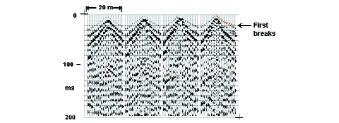
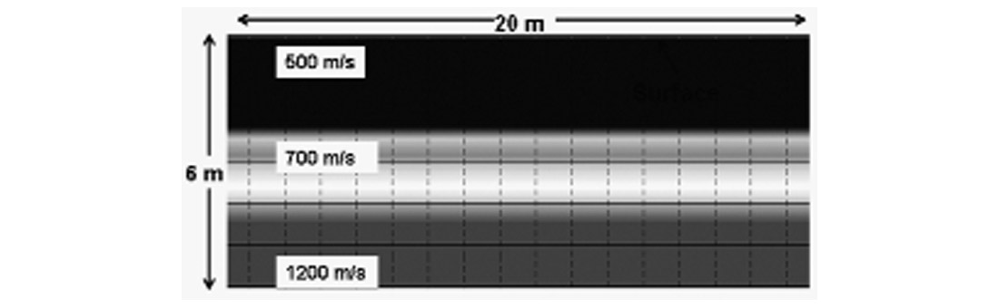
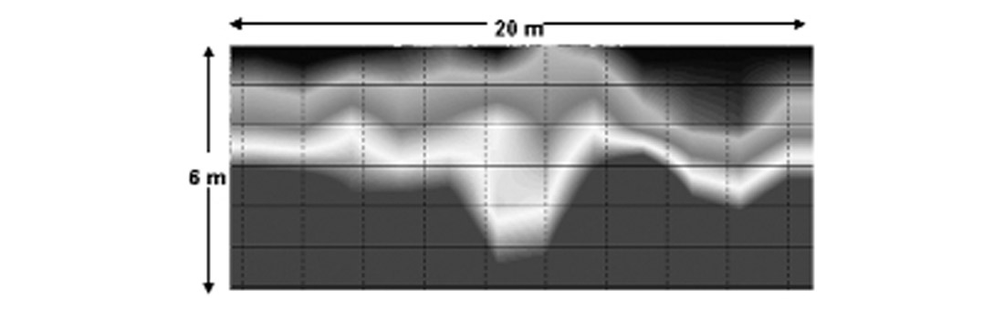
To verify the anomaly on the 2001 reflection image with other observations, we carefully picked the first breaks on all 420 traces in the 2001 survey in order to use transmission tomographic techniques. As can be seen in Figure 6, there is no clear pattern in the first breaks to suggest a discretely layered model of the near surface so we decided to use the ‘turning ray’ model, which assumes no particular layering, but only a smooth velocity increase with depth. We constructed such a model (Figure 8) based on measurements of first arrival velocity and stacking velocities, and traced rays through it to provide model times with which to compare the first break pick times. The tomographic approach we adopted uses the time differences between first breaks and model rays to estimate velocity changes necessary in model cells traversed by the raypaths to better fit the measured pick times. The raypaths remain fixed in the interest of stability, so the resulting image is considered a first order approximation only. Figure 9 is the tomographic image resulting from the starting model of Figure 8 and the carefully edited first break time picks. Of great interest, particularly when compared with the anomaly on the rescaled reflection image in Figure 10, is the trench-like tomographic anomaly. Since these results, from essentially independent data sets, tell a similar story, the anomaly assumes greater credibility.

More ruins, anyone?

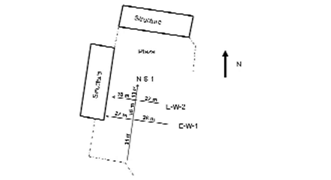
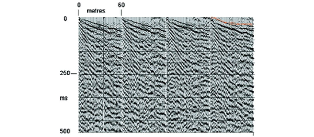
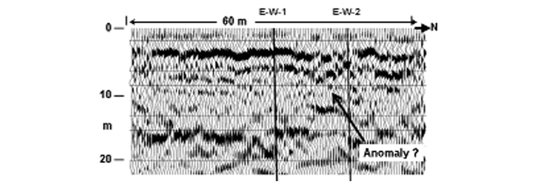
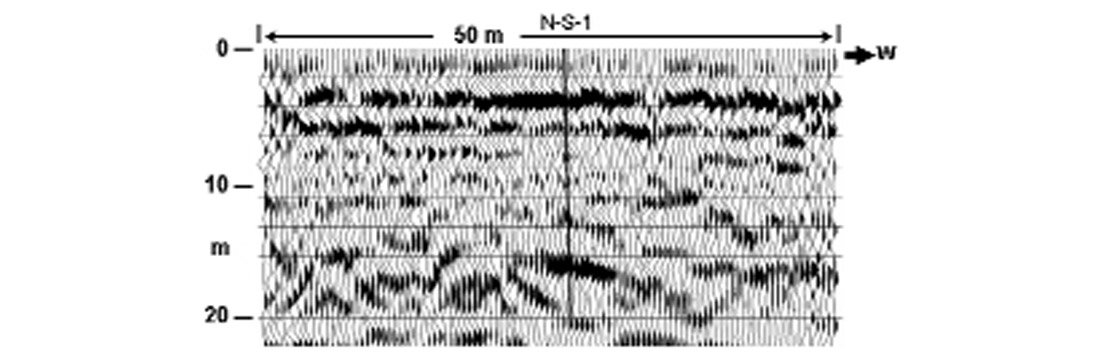
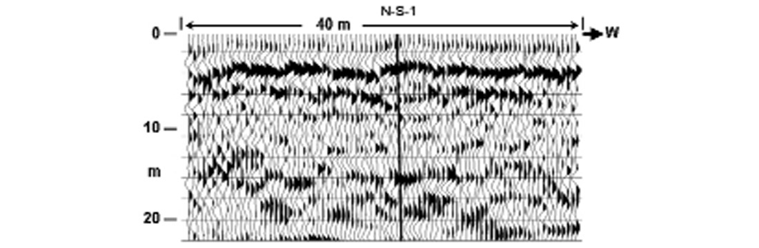
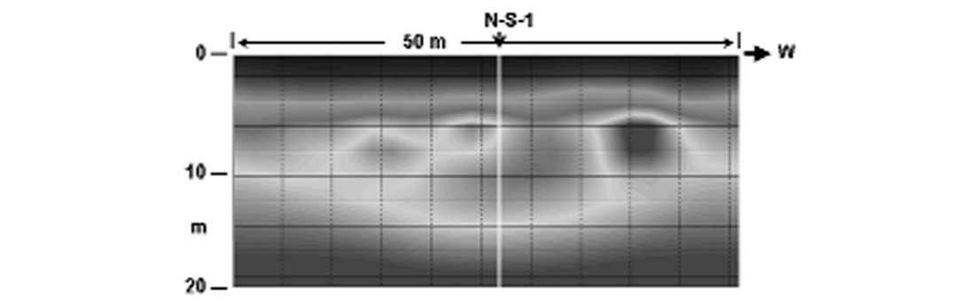
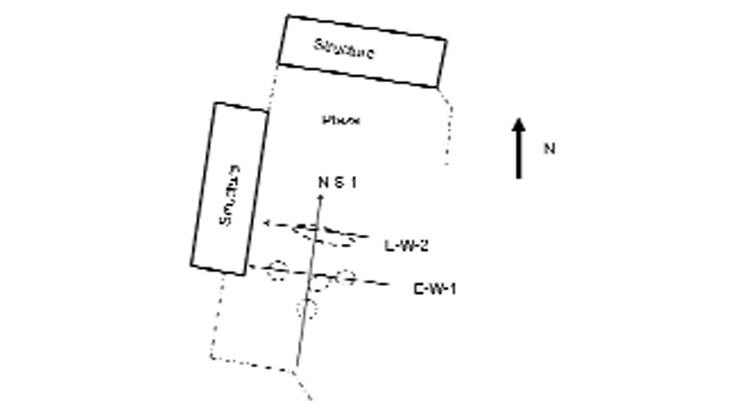
The final set of archaeological seismic data to be discussed was obtained in 2002 at Ma’ax Na, a second Mayan temple site in Belize. Three intersecting lines were laid out in a plaza region adjacent to existing structures (Figure 11). The technique used on each of the lines was similar to that used in the 2001 Chan Chich survey, except that all three lines had many more stations (40, 50 and 60 stations). Once again, 1 metre station spacing was adopted and the source was a single hammer blow, with source stations between the receiver stations. Figure 12 shows typical source gathers for the 60 station line N-S-1. Source-generated noise is a problem on these lines, as at Chan Chich, but careful processing leads to reflection images in Figures 13 to 15. The line intersections are indicated on each of these sections and it can be verified that the lines all tie well in reflection time and character. Once again, however, the shallowest reflection, corresponding to the bedrock surface, is not as trustworthy as we would prefer because of the low stack fold and the careful muting used to eliminate interfering refractions. The most obvious anomaly on the three lines is the one marked just right of centre on line N-S-1 in Figure 13.

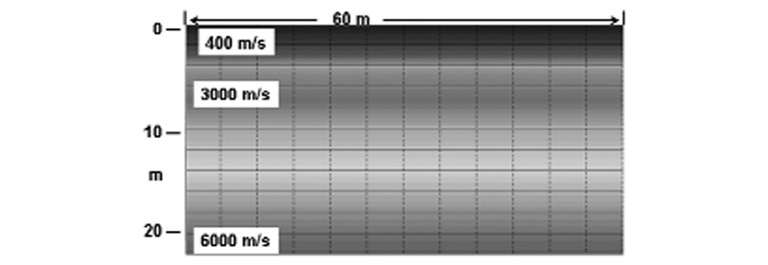
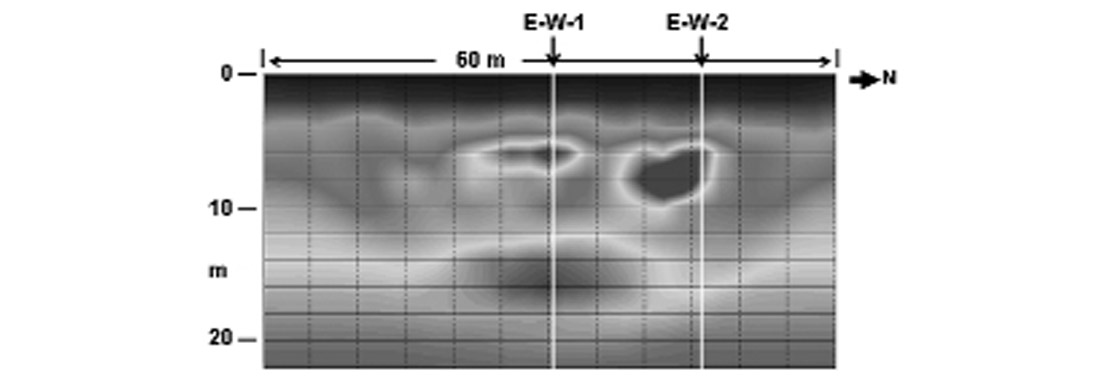
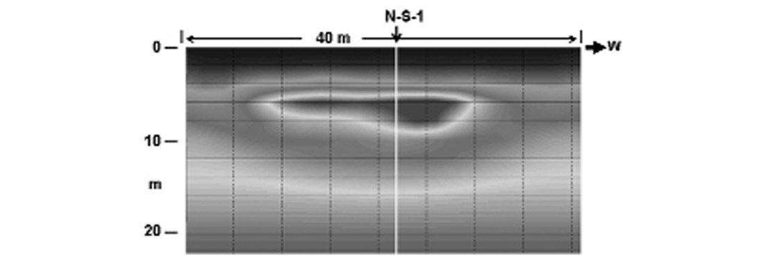
Following the procedure established for the Chan Chich 2001 data, we decided to attempt first break turning ray tomography on the three Ma’ax Na lines as well. Because there are far more data on each of these lines than on either of the Chan Chich lines, there are correspondingly more first break picks to make (and to edit) for each of the lines (3660, 2550 and 1640). Consequently, the images shown here correspond only to tomography performed with unedited picks. Although as many as 40% of all the picks may need editing, the mispicks appear to be random; so their influence on the image is small, except to decrease the image contrast. Figure 16 is the starting model for the turning ray solution at Ma’ax Na, while Figures 17-19 are the tomographic images corresponding to lines N-S-1, E-W-1 and E-W-2, respectively. Interestingly, we see that these images tie as well as the reflection images; wherever a line intersects a ‘hard’ anomaly, a corresponding crossline exhibits the same anomaly. In contrast to Chan Chich, at Ma’ax Na correlations between velocity anomalies imaged by tomography and the details of the reflection images are more subtle, except for the most prominent ‘hard’ anomaly shown on line N-S-1. The hard anomalies may not exhibit the abrupt vertical acoustic contrast necessary for strong reflections and they appear not to interrupt significant reflection interfaces.

In Figure 20 the various ‘hard’ anomalies are plotted on the site map for Ma’ax Na. We speculate that they may correspond to portions of older structures buried under the more recent rubble in the plaza. Only time (and digging) will tell.

What’s Real and What’s Not

It’s interesting to produce suggestive images and maps of subsurface anomalies that may be related to archaeological features but the bottom line is how well the images correspond to actual subsurface features. At the present time, none of the anomalies at either Chan Chich or Ma’ax Na has been verified by excavation although the images have been presented to archaeologists on site who are seriously considering them. Until such a time as we have verification of actual archaeological features discovered with the aid of seismic techniques, we will continue to develop and test shallow seismic imaging methods, and to speculate. Our hope is that, someday, Indiana Jones will be persuaded to trade in his bullwhip for a sledgehammer.

Acknowledgements

The author gratefully acknowledges Rob Stewart for initiating the whole investigation into archaeological uses of seismic techniques, for providing the data from both the Chan Chich and Ma’ax Na sites and for discussion and guidance. In addition, the following persons and institutions should be prominently acknowledged: Drs. Claire Allum & Leslie Shaw (Bowdoin College, Maine), Dr. Eleanor King (Howard University & Ma’ax Na Archaeological Project), Dr. Jaime Ave (Dept. of Archaeology, Govt. of Belize), Dr. Fred Valdez Jr. (U. of Texas at Austin), Eric Gallant and Henry Bland of CREWES, Richard Xu (CGG/UofC) and Rob Birch (UofC).

Indiana Jones and all related indicia are trademarks of & copyright © Lucasfilm Ltd.