In the Foothills, Prestack Depth Migration IS Interpretive Processing

Introduction

In the Foothills of the Canadian Rocky Mountains, explorationists face a wide spectrum of challenges, ranging from economic ("Is my prospect large enough to justify a multi-million dollar well?" "Can hydrocarbons be transported from the well to the market inexpensively?") to technical ("Can I map my structure using seismic data?" "Can I produce an interpretable seismic section that will help me choose a well location?"). In this paper, we shall concentrate on the technical end of the spectrum, in particular on the final of these questions. We shall offer evidence to support the point of view that prestack depth migration is the most powerful seismic processing tool available to the interpreter working in the Foothills. The use of this tool, however, is far from automatic; rather than leading to an unambiguous conclusion about geologic structure, it is interpretational, allowing (indeed, requiring) the interpreter to choose from among different structural hypotheses.

In this paper, we shall first try to place pres tack depth migration into a broader context by reviewing the imaging methods available for the past few decades, emphasizing the fact that methods used in the past have approximated the action of prestack depth migration to some degree. Second, we shall discuss the problem of statics, which affects the quality of seismic images obtained in the Foothills in several different ways. Third, we shall address the dual problems of imaging and velocity estimation. By showing some modern methods for estimating velocities for prestack migration, both time and depth, we hope to dispel the myth that estimating migration velocities is necessarily a boring and time-consuming task.

The Need for Prestack Migration in the Foothills

A brief history of seismic imaging

In the 1960's, the combination of high fold (on the order of ten!) and the vertical stacking of NMO-corrected CDP records allowed superior imaging and noise attenuation than had previously been possible. This process is essentially the same as migrating all the traces in a CDP record to the midpoint location with a zero-dip migration operator. Crude as it is, this process still produced interpretable images of flat-lying structures, and was adequate for imaging the layer-cake geology of, say, Eastern Alberta. For dipping structures, a CDP stacked section produced a distorted subsurface image for two reasons. First, dipping layers appeared laterally shifted from their true positions in a systematic way; second, dipping layers were attenuated, or washed out, on the stacked section. The lateral positioning of events by the time migration methods of the 1970's corrected the first of these problems (though only to a degree), improving the interpretability of a stacked section. The lateral positioning of events by the time migration methods of the' 1970's was not perfect because these methods used a fairly crude approximation (RMS velocities) to the actual interval velocity field required for accurate, precise imaging. The development of DMO in the 1980's corrected the second distortion of NMO/stack, namely the attenuation of steeply dipping events, at least where lateral velocity variations are not too severe. DMO accomplishes this by effectively transforming a nonzero-offset section to a zero-offset section using an operator that honors all dips. The processing sequence NMO/DMO/stack/migration typically produced more accurate and interpretable images than the sequence NMO/stack/migration. However, time migration, by its use of an inaccurate and imprecise velocity field, impedes an interpretation of the precision that is needed to pinpoint some of the small-scale horizons that are the drilling targets in the Foothills. The development of depth migration methods, which use an interval velocity field to define the migration operator, in the 1980' s partially overcame this problem, but exposed a more fundamental problem associated with the cascade of a number of imaging steps (NMO/DMO/stack) before migration. The weak link in this processing chain is NMO/stack, with its assumptions of flat reflector geometry and hyperbolic moveout. These assumptions, which have proved so reliable and robust for imaging in even moderately complicated reflector geometries, break down completely when they are applied to data from areas with the structural and topographic complexity of the Canadian Foothills. Thus, the need for migration before stack, which avoids the problem of migrating a stacked section whose events have been compromised by the unrealistic assumptions of NMO/stack.

When we stop to reflect for a moment, we realize that prestack migration, in time or depth, does what NMO/stack tried to do more than thirty years ago, but couldn't for reasons purely computational. Mechanical migration was available several years before NMO/stack, and undoubtedly would have evolved quickly into digital prestack migration if the computational horsepower had been available in the 1960' s. Since it wasn't, a complicated processing flow of imaging processes was used to approximate a simple single process of migrating data directly from recorded field records, after a minimal amount of preprocessing. It's easy to forget this fact, and we sometimes prefer to use the familiar set of approximate processes over the single, inherently better, process. (In fact, an expert seismic data processor can often produce a much "nicer" migrated section for interpretation by using the tried-and-true NMOIDMO/stack/migration flow than an interpreter can produce by using the simpler, single-step prestack migration process. The reason for this is, in a word, velocity. Each of the imaging processes NMO, DMO, poststack migration, and prestack migration involves the choice of a set of velocities. By using different, possibly unrelated and unphysical, sets of velocities for NMO, DMO, and migration, a skilled processor can coax events through the processing flow all the way to the final migrated stack that an interpreter will be hard-pressed to duplicate by performing velocity analysis after migration but before stack. But this situation is changing; prestack migration velocity analysis is becoming easier to apply and more reliable, as we shall show.)

An imaging comparison

It should be clear by now that we should image our seismic data using the most accurate and powerful methods available. Seismic imaging should be constrained only by seismic wave behavior, allowing accurate lateral positioning of reflection events and accurate depth conversion. We should therefore use prestack depth migration (from topography, anisotropically, and in three dimensions, of course!), and we should use the actual near-surface and subsurface interval velocities to guide the wave propagation through the Earth. On the other hand, seismic imaging in the Foothills is heavily constrained by issues such as data quality, economics, and perceptions. All of these are important constraints, and they are all related. For example, the economics of a prospect often dictate that an interpreter is responsible for land capture, as well as seismic acquisition, processing and interpretation, with heavy time constraints to arriving at a drilling decision. Under such pressure, only a very brave interpreter will commit the perceived, if not real, extra time needed for prestack depth migrating one or more lines over the prospect. If the interpreter has access to a skilled processor and standard imaging technology, the temptation to yield the processing responsibility will be great.

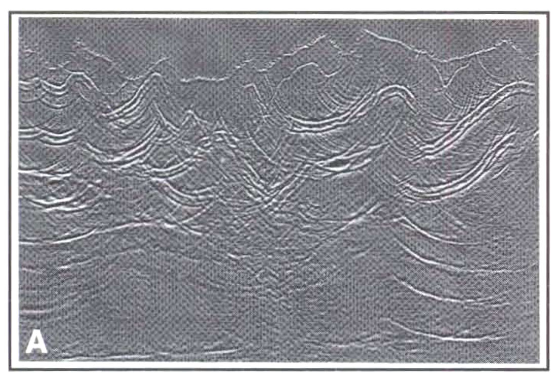
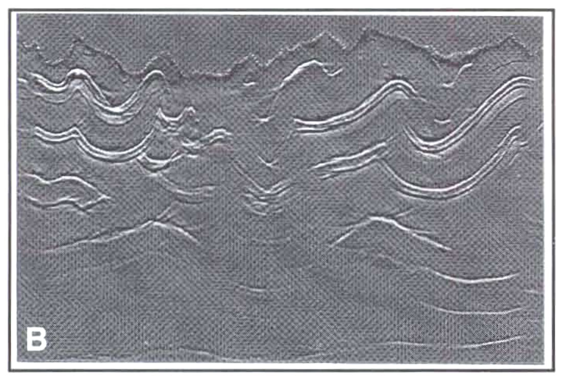
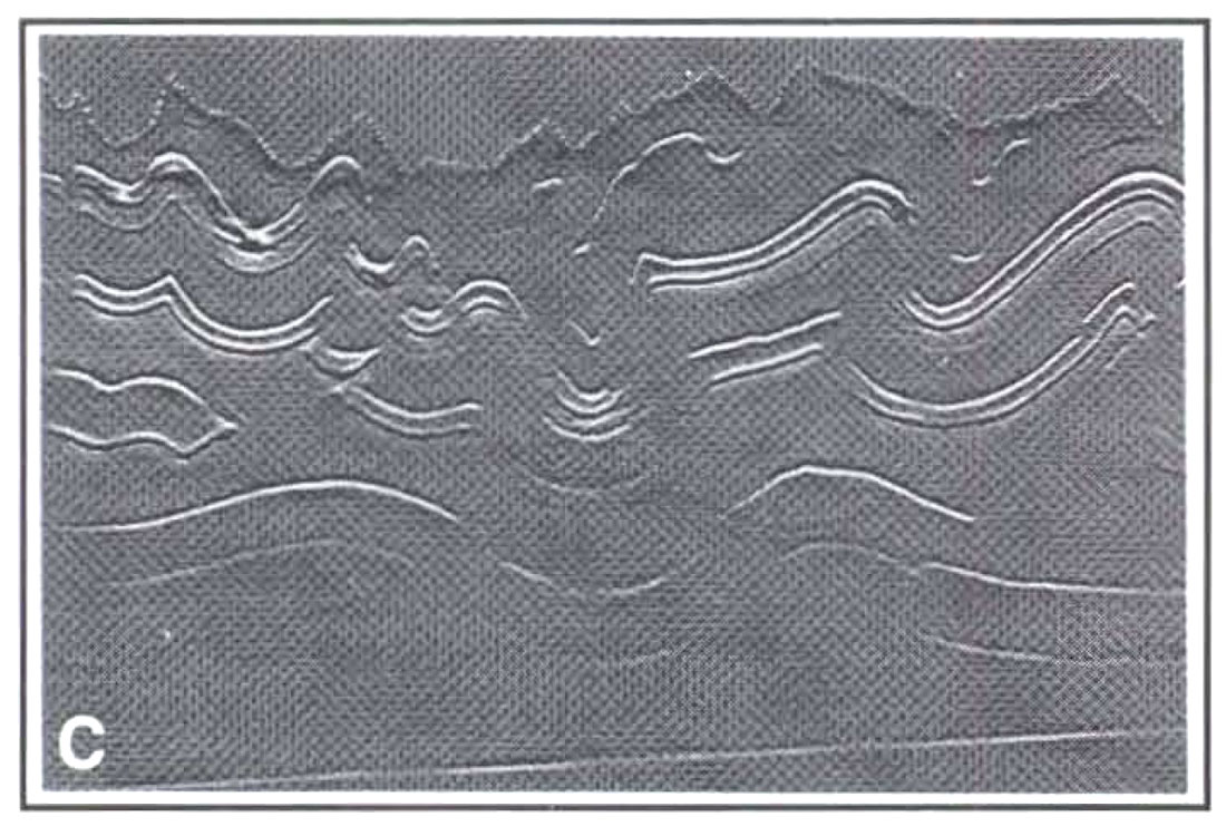
As the following somewhat biased example shows, however, the price for doing this might be unexpectedly high. Figure1 shows three stacks from a synthetic (acoustic finite-difference data set that has been used to model seismic wave propagation in northeastern British Columbia. Figure lea) shows a poststack depth migration, where an expert processor has performed NMOIDMO/stack. The migration was performed from topography, and it used the actual interval velocities. Figure I(b) shows a prestack time migration, also from topography, using migration velocities that were derived from the actual velocities. Figure I (c) shows a prestack depth migration from topography, using the actual interval velocities. Clearly, the prestack depth migration has produced the best image; we would be very surprised otherwise. What we do find surprising is the high noise level on the poststack migration. This is due in part to the lack of random noise on the original shot records, resulting in an artificially high standout of coherent noise (edge effects, multiples, etc.) on the standard-processed stack that the extra operations of prestack migration have cancelled out. Looking past the coherent noise, however, it is still hard to make structural sense of much of Figure lea), for example in the nested synclines in the middle of the section. Also, the deeper anticline on the right side of the model (a possible drilling target) is obscure. Much of the confusion on the poststack migration has been cleared up by the prestack time migration, which has made the interpretation relatively straightforward. However, some problems remain on Figure l(b). In depth, the basement reflector is known to have a constant dip, but this is not at all what we observe on the prestack time migration. Can we convert the time section to depth with any confidence? How much relief really exists on our possible drilling target on the right side of the section? Performing prestack depth migration shown in Figure l(c) has, in addition to clearing up the small amount of residual noise present on the time migrated section, solved the depth conversion problem. Of course, we used the actual migration velocities to perform the prestack depth migration but, in general, we must estimate those velocities somehow. With a poor estimate of the interval velocities, our depth migrated image will be poorly focussed and structurally wrong. But if we can estimate velocities reliably (and we contend that we can often do just that), our prestack depth migrated image will be at least as interpretable as our pres tack time migrated image, with a smaller risk of lateral and vertical positioning error.

A final note about both of the prestack migrated sections: Some of the very steeply dipping anticlinal flanks have not been satisfactorily imaged. This is due not to an inherent inability of the migration program to image steep dips, but rather to our choice of an inadequate migration aperture. Processors are well aware that parameters such as migration aperture can have a major effect on the quality and interpretability of a processed section; interpreters who do not process seismic data are not usually so aware of this fact. So interpreters should be very nice to their processors.

With our example, we have shown that prestack migration can produce a clearer image than poststack migration, and that pres tack depth migration provides more accurate lateral positioning and depth conversion of events than prestack time migration. Present-day Foothills exploration targets lie under more complicated overburden than targets from even five years ago, and thus demand high-quality imaging more than previous targets did. Since drilling results produce the ultimate interpretation of a prospect, it is greatly in the interpreter's interest to predict the geologic structure that the drill bit will encounter as accurately as possible.

Statics

Statics is an important component of imaging, but statics is a big subject, far too big to receive only the most cursory treatment in this paper. We shall mention refraction and residual statics and their relationship with imaging only in passing, and we shall show by example the effects of properly using elevation statics information with prestack depth migration.

"Statics" typically means the time shift of traces within a record in order to improve the lateral continuity of the record. Statics problems and solutions come in many flavors; first, we mention refraction and residual statics. These methods have two objectives: (l) to improve data quality, especially in the near-surface (so that near-surface reflectors can be imaged better); and (2) to estimate near-surface velocities. It has been our experience that the problem of inverting refraction data for near-surface velocities is horribly ill-posed, so that statics usually fails to find the correct velocity field. (Others will disagree with us; they have had good success in using the velocities from statics in generating a near-surface model. Our hat is off to those skilled practitioners of the art of statics.) It has also been our experience that applying the statics improves the data quality significantly, and that the replacement velocity used in the statics application provides a useful near-surface velocity field. (Others will disagree here also, and, again, we tip our hat).

Elevations provide another "statics" problem. In order to insert topography variations into imaging processes, some sort of topographic correction must often be applied to the data before imaging. The simplest elevation statics correction for migration is to migrate directly from topography. However, not all migration methods allow this in a convenient fashion. For example, finite-difference migration requires that seismic traces be downward continued into the Earth from a flat datum. But the traces weren't recorded on a flat datum! In order to get them there, we might time shift the traces by a certain amount to approximate the upward shift of the source and receiver locations from the actual acquisition surface to the datum. Alternatively, we might use a wave-equation process ("wave-equation datuming," introduced in 1979 by Berryhill), which moves an entire recording spread from the acquisition surface upward to the datum in a fashion consistent with the wave equation. In some instances, performing elevation corrections by static shifts might approximate the more expensive but valid wave-equation datuming reasonably well, but where topographic variations are significant, this use of static shifts can seriously compromise the accuracy of the final migrated image. especially in the near-surface. For example, consider Figures 2 and 3, which show the application of the two different elevation correction methods on a portion of our earlier example. In Figure 2(a), zero-offset data were static shifted from the acquisition surface (the black line) to a datum above the topography, and in Figure 2(b), the traces were datumed using the wave equation. Figures 2(a) and 2(b) show significant differences from each other; clearly, migrating these two sections from the flat datum will result in very different images. These images are shown in Figure 3(a) and (b), which correspond to the unmigrated images in Figures 2(a) and 2(b), respectively. Both migrations were performed using the actual subsurface velocities below topography and the replacement velocity above topography. Figure 3(a) shows near-surface overmigration artifacts that characteristically result from performing elevation corrections by static shifts followed by migration and using actual velocities. Figure 3(b) agrees almost perfectly with a zero-offset migration performed directly from topography; it is the more correct image.

As this example shows, it is preferable to migrate directly from topography, or at least to perform elevation statics before migration in a way that is consistent with the wave equation. As a side note, wave-equation datuming is useful for more than preparing data for a migration algorithm that must be implemented from a flat datum. It can be also used to prepare data for other processing methods such as planewave decomposition. Expressing seismic data in the plane-wave domain gives us access to a number of powerful processing techniques that are more naturally formulated for plane-wave records than for shot records, for example predictive deconvolution. Prestack migration can even be performed in the plane-wave domain, with some interesting consequences for velocity analysis.

Imaging and Velocity Estimation

The Foothills of the Canadian Rockies contain extreme topographic relief, very complicated geologic structures and, especially in the vicinity of fast carbonate rocks, rapid lateral velocity variations. We have seen the ability of prestack depth migration to image complicated structures from topography with accuracy and precision, both vertically and laterally. Such accuracy and precision are needed in determining the correct drilling location and in computing the volume of hydrocarbons present in a structure. There is a catch, though. In order to produce this accurate, precise image of the Earth's subsurface, we need to know the propagation (interval) velocities. But away from wells, we have only a vague idea of the velocities, which can be made precise only from prestack depth migration velocity analysis. So, in order to image accurately and precisely, we need accurate, precise knowledge of the velocities; and in order to obtain accurate, precise knowledge of the velocities, we need to image accurately and precisely. This is the central problem of pres tack depth migration that, until recently, has greatly limited the success of prestack depth migration in areas of poor velocity control. In the past few years, however, some workers have made substantial progress on this problem. We shall describe this progress, but first we shall discuss some alternative velocity analysis methods.

First, let us distinguish between poststack and prestack migration velocity analysis, and between time and depth migration velocity analysis. Velocity analysis for poststack migration has largely been performed before stack, during NMO and DMO. We can perform repeated poststack migrations on a stacked section using different migration velocity functions, changing the geometric relationship of the migrated events, but events will not appear and disappear as they will on repeated prestack migrations. This is because poststack migration will migrate all the events that have survived NMO/DMO/stack. Perhaps surprisingly, there are advantages to this approach when it is used by a very proficient processor. One velocity function might be used to perform the NMO corrections, a second to perform the DMO corrections, and a third to perform the migration, with each of the first two functions carefully chosen to maximize the energy of selected events. Although this approach can seriously compromise our ability to convert the final section to depth (even if the poststack migration is a depth migration), it can insure that all reflection events show up on the final migration, even the out-of-plane events. However, in the hands of a less-than-expert processor, this approach puts us at the mercy of the stack. If an event hasn't been stacked, it won't magically appear on the migrated section. On the other hand, prestack migration velocity analysis is typically performed after migration but before stack. (This is not necessarily the case, however, and we shall show an example of prestack time migration velocity estimation performed after stack.) Performing the velocity analysis after migration is preferable in principle to performing it after the approximate procedures of NMO and DMO, but it is not as flexible, and it can lock us into analyzing data with a substantial part of the reflection information removed.

Prestack time migration velocity analysis concentrates on finding the appropriate imaging velocity function, while prestack depth migration concentrates on finding the correct interval velocity function. We know what interval velocity means, but what is imaging velocity? Imaging velocity is merely the numerical value of velocity that, at an (x,t) point in the migrated section, produces a better image than any other value for velocity. For example, if we perform a number of constant-velocity prestack time migrations and view all the migrated stacked sections, a particular horizon will be imaged best at one of the velocities; that velocity is the imaging velocity for the horizon. Imaging velocity, then, is the prestack migration version of DMO/stacking velocity. Like DMO/stacking velocity, imaging velocity is extremely useful for producing an interpretable stack, and practically useless for depth conversion in areas where the velocity varies laterally. Interval velocity, on the other hand, provides both the imaging velocity for prestack depth migration and the velocity field which expresses the migrated stack in depth. Estimating interval velocities for prestack depth migration is a more ambitious and more rewarding undertaking than estimating imaging velocities for prestack time migration, but the latter operation is usually easier.

Prestack time migration velocity analysis

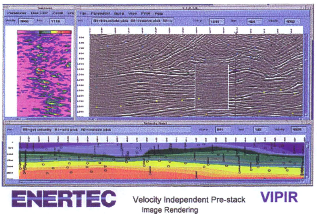
We next describe some promising methods for using prestack migration to estimate velocities. First, prestack time migration. As we mentioned, prestack time migration seeks the velocity function that produces the best stack at every point in the migrated section. One method for doing this has been around for a number of years; Enertec has developed an interactive, workstation- based version that allows an interpreter to view the imaging velocity function as it is being built. We thank Keith Wilkinson for providing this example, which is shown in Figure 4. This figure shows a prestack migrated section in one window of a workstation screen, with a subwindow in which the image quality is poorer than elsewhere. The subwindow is the region of analysis; forty to fifty prestack migrated subsections are animated within than subwindow of (x,t) migrated space. As the velocity approaches the correct imaging velocity for an event in -that subwindow, the image quality improves. In Figure 4, the subwindow shows a migration with a velocity far from the correct imaging velocity. When the correct imaging velocity is reached at an (x,t) location in the subwindow, the interpreter selects that velocity at that point. Different points in the analysis subwindow will have different imaging velocities corresponding to the different colored picks covering the section; the cloud of (x,t) points along with their corresponding imaging velocities is registered in the window below the migrated section; the color variation shows the interpolated imaging velocity function. Alternatively, the interpreter might prefer to pick spectra; the spectra to the left of the migrated section refers to a single migrated location (the one denoted by the vertical line near location #1047). The spectrum plot shows migrated strength as a function of velocity, with clearly visible peaks, corresponding to a velocity that increases with depth. Where reflection quality is good, both of these approaches are very fast, easy, and accurate ways to find imaging velocity for prestack time migration. Even where the data quality is poor, these interactive approaches enable the interpreter to determine imaging velocities for prestack migration, with the ultimate goal of producing the "best" migrated section, more conveniently than other methods.

Prestack depth migration velocity analysis

Next, we discuss the problem of prestack depth migration velocity estimation. We have implied that this problem is fundamentally more difficult than the other velocity analysis problems and, indeed, this is so. In prestack time migration, it is enough to find the correct imaging velocity at each (x,t) point on the stack independently of the rest of the points. In prestack depth migration, however, we want to find the correct interval velocity at every (x,z) point on the stack, but our choice for interval velocity at anyone point affects our choice at a huge number of points near that point. This is because a change in the interval velocity value in one small cell will affect wave propagation, and the calculation of traveltimes by depth migration program, not only within that cell, but in all cells in an expanding cone beneath the cell in question. So typically, we must first estimate the interval velocity function in the shallow part of the section before we can estimate deeper velocities, a process called "layer stripping." Contributing to the difficulty of this approach is the fact that, for common-shot and common-offset migration, migrated CDP gathers are more heavily muted at shallow depths, and velocity estimation depends on our ability to detect residual moveout at these depths over just a few traces.

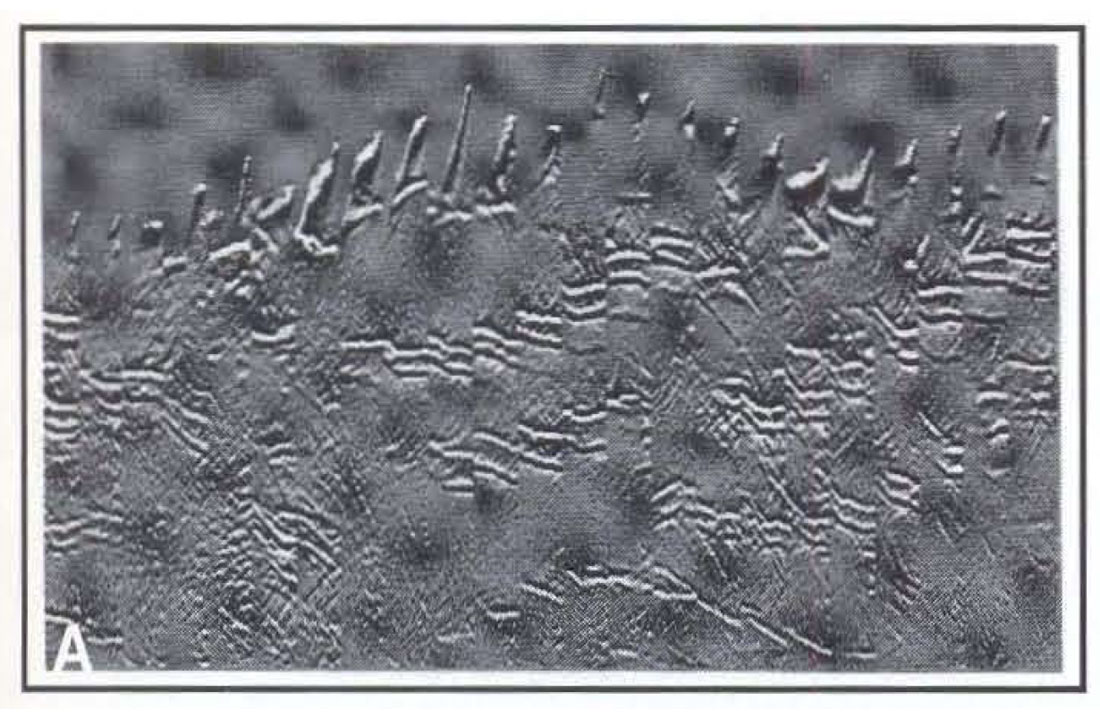
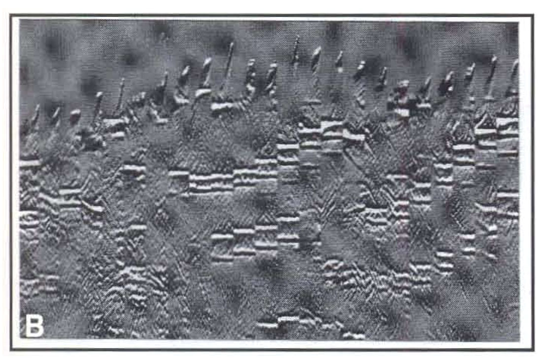
The traditional method of prestack depth migration velocity analysis has been to detect residual moveout on migrated CDP gathers, and estimate by guessing the amount of interval velocity change needed to flatten, or remove that residual moveout from, those gathers in the next iteration of prestack migration. Figure S illustrates that approach, and hints at its difficulty. In Figure Sea), we show a set of migrated CDP gathers from our earlier synthetic example, where we used an interval velocity function for migration that was ten percent too low everywhere, and in Figure 5(b), we show the same set of gathers where the migration velocity function was correct. Clearly, the shape of the residual moveout in Figure Sea) indicates that the interval velocities need to be changed before the next migration iteration, but by how much? Even in this example, where the same percentage increase needs to be applied to the interval velocity in all the cells, the answer is far from obvious. Layer stripping, starting with the migrated gathers in Figure 5(a), might lead to the correct velocity after a number of pres tack migration iterations by an expert processing interpreter. Just as likely, even an expert will decide on incorrect velocities in at least some parts of the section, and these errors will be compounded, causing compensating errors deeper in the section.

Fortunately, some velocity estimation methods have been developed that improve on the traditional approach. The first of these is called tomography, which is an automatic method. There are a number of different approaches to tomography, and we will describe one of them. First, residual moveout is picked on unmigrated gathers. (Actually, it is much easier to pick on a stack and propagate the picks automatically through unmigrated common-offset records. A CDP sort of those records will show the picks on the gathers.) Then, using ray paths through the present velocity model, source-to-reflector-to-receiver traveltimes are computed, yielding values that are typically different from those picked on the gathers. These differences are assembled into a large vector, and a linearized version of the ray equations provides a large matrix equation involving the traveltime differences, raypath length through all the cells in the velocity model, and velocity updates. This equation is solved by least-squares methods for the velocity updates. which tell us how much to change the velocity value in each cell before the next iteration. It is possible to introduce constraints, such as well velocities, into this procedure. Another version of tomography works in the migrated domain, minimizing residual moveout on migrated gathers. The procedure is different, but the mathematics is very similar to the version we've described.

Tomography is automatic, and it is global (rather than layer stripping, it updates all the velocities at once). It aims to minimize traveltime differences, and it does a very good job at that. Unconstrained, it can produce "blobby" velocity models that do not appear to honor geologic boundaries, but it can be constrained to honor geologic boundaries. Although it is automatic, its use of least-squares inversion methods requires the user (the interpreter?) to input parameters related to the mathematical properties of matrix algebra, and the user might feel uncomfortable doing this. Also, the unconstrained use of tomography can lead to migrated sections with visible long-wavelength structural artifacts. In the hands of an expert, however, tomography can produce geologically reasonable prestack depth migrated sections with very little residual moveout in the CDP gathers in a very small number (one to three) of iterations.

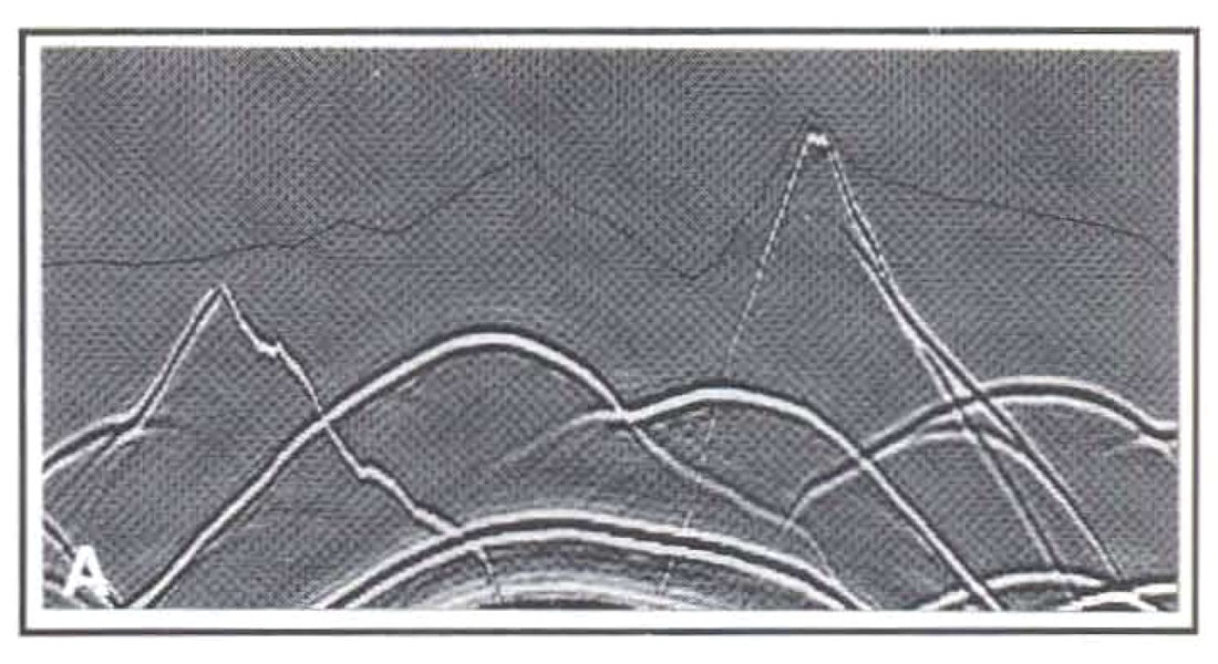
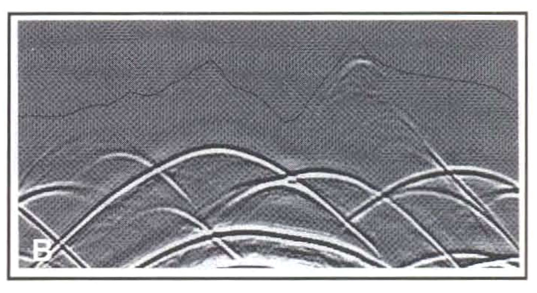
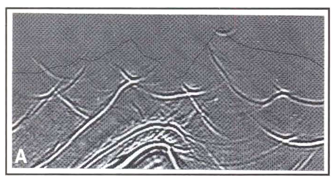
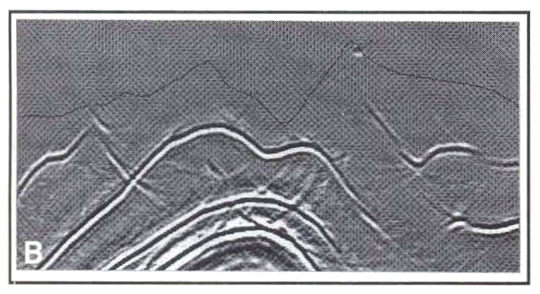
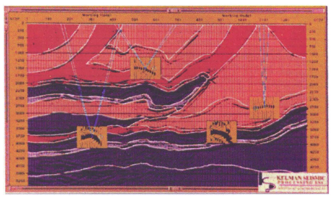
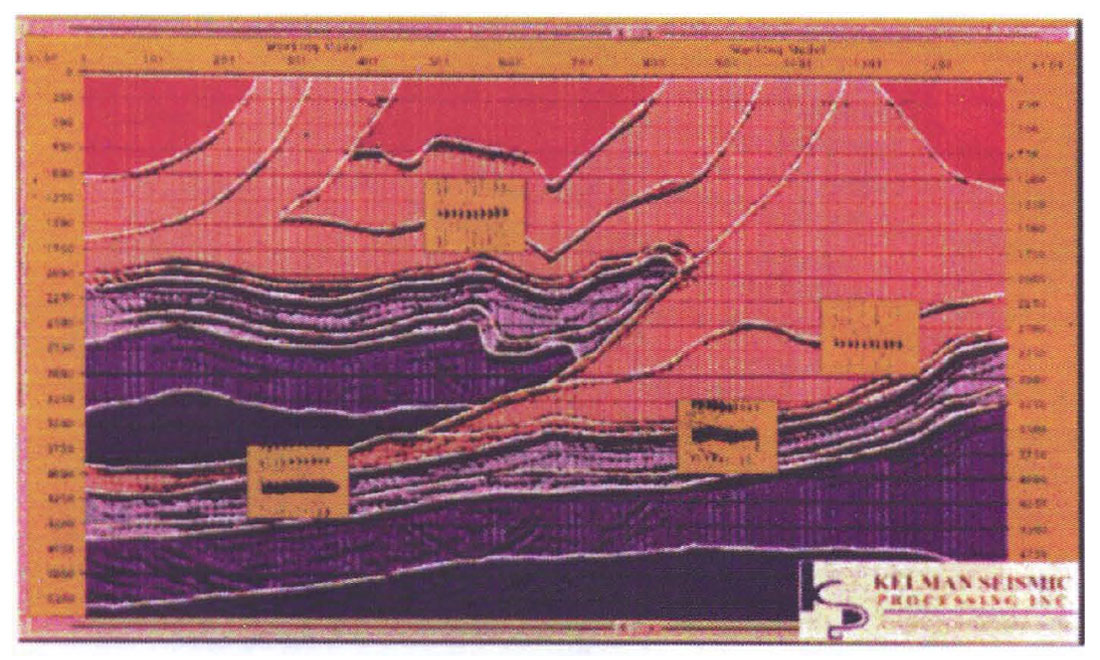
A more recently developed method might be called "specular tomography." We describe a version that was developed by Kelman, and we thank Ron Schmid for providing us with an example, illustrated in Figure 6. This method, rather than attempting to flatten migrated CDP gathers all at once, concentrates on one gather at a time. it starts with an interval velocity model, a stack, and migrated CDP gathers from a prestack depth migration iteration. Picking an (x,z) point with some reflection energy on the migrated stack (Figure 6(a) calls up the gather from that location, as well as raypaths from the reflection point through the velocity model. Those raypaths (the faint white lines in Figure 6(a) show the portions of the velocity model traversed by the seismic energy corresponding to a particular offset. For the shallowest gather in Figure 6(a), the seismic energy for most of the offsets has travelled through the two velocity bodies immediately above the reflector. So, to flatten the gather on the next migration iteration, the velocity needs to be decreased in one or both of those bodies. If, say, the velocity in the upper body has previously been determined to be correct, a residual NMO calculation is performed interactively, without remigrating, by entering a new value for velocity in the lower body. The velocity value that flattens the CDP gather will be used in the next migration iteration. Proceeding from the top down allows the velocity in the top bodies to be fixed first, so that residual moveout encountered in later iterations can be attributed to deeper bodies. Figure 6(b) shows the stack and selected migrated gathers from the final iteration of this process.

This procedure eliminates the need for guessing a value for velocity in the next migration iteration by the residual NMO calculation, which allows the interpreter to preview the effects of a guess interactively. The guess might not be correct - it might not exactly flatten the gather after the next migration iteration - but it is almost always a step in the right direction. This approach involves the interpreter more than tomography does; it forces him/her both to judge between conflicting information on the migrated gathers and to update the velocities manually. The authors' preference is in this direction. We believe that involving the interpreter in this way allows a great flexibility in testing geologic hypotheses that is not so easily available from tomography. Because this process is not as automatic as tomography, it might require a few more migration iterations. But it still promises to reduce the number of iterations considerably from the traditional method of guessing a velocity value and remigrating.

To summarize: several years ago, velocity analysis for prestack depth migration was tedious and time-consuming, and there was no assurance that iterative migration and velocity estimation would converge to a solution. Today, however, at least two methods allow faster, easier, and more accurate velocity estimation. The two methods are focussed differently: tomography is oriented more toward processing experts, while "specular tomography" is oriented more toward interpreters.

Conclusions

In the oil and gas industry, geophysicists are unique in their time-domain view of the earth. From our point of view as geophysicists, this time-domain view is natural enough, since seismic data are recorded in time and have historically been processed in time. However, to communicate with geologists and drillers, we need to be able to transform this view of the earth to a depth-domain view. Historically, this has presented a great challenge to geophysicists but, as we've shown in this paper, recent advances in velocity analysis methods, coupled with access to unprecedented computational horsepower, have placed this goal within our grasp. As a sidelight of the advances in computational power over the past decade, prestack time migration is also widely available to produce a more interpretable image than the one produced by the standard processing flow of NMO/DMO/stack/poststack migration. But at the end of the day, the traditional interpretational scheme of applying the colored pencils to time-migrated sections must eventually give way to estimating velocities for prestack depth migration interactively on interpretation workstations, for the ultimate purpose of placing wells in the correct vertical and lateral position.

With increasing pressure being placed on geoscientists to find hydrocarbons in difficult areas under tough economic conditions, one of the solutions is to turn to technology for assistance. The ultimate technological solution presented in this paper, prestack depth migration, places the power of imaging and velocity analysis in the hands of the interpreter, and it does so without the approximations that have compromised geophysicists' confidence in the precision of their structural interpretations. Prestack depth migration has been viewed by many as an unfriendly technology, but recent advances in computing power and velocity analysis techniques have made this technology more accessible to seismic interpreters than ever before. We believe that the combination of the increased accessibility of imaging technology and the risks associated with drilling Foothills targets justifies the routine application of prestack depth migration as an interpretational tool.

Acknowledgements

We wish to thank Enertec Geophysical Services and Kelman Seismic Processing for providing us with data examples. We also thank Randy Cameron for lending his processing expertise, and Allan Powers for held in preparing the figures.