Improved trending of features on aeromagnetic maps

Summary

In mining and near-surface geophysics, aeromagnetic maps are an important tool for mapping geology. In some terrains, the geology is comprised of narrow features striking at multiple angles. When the aeromagnetic data is converted to a grid, these features do not always image well, particularly when the features are not perpendicular to the flight lines. A new tool, utilizing anisotropic diffusion filters, has recently been developed to deal with this problem. The tool provides good images of the aeromagnetic data, but when the grids are converted to derivative maps such as the analytic signal, artifacts appear along the flight lines. We have made a further improvement to the new tool that removes these artifacts and produces well trended images on both the aeromagnetic maps and the derivative maps. The method compares favorably with other methods for trending aeromagnetic maps.

Introduction

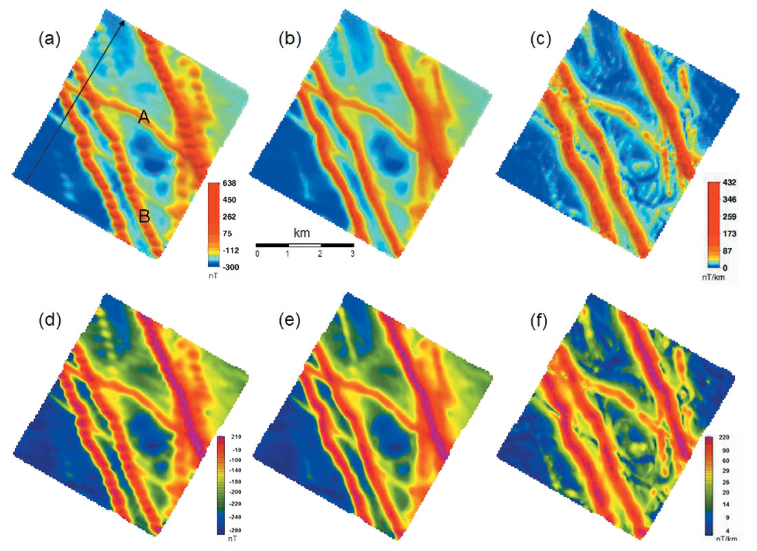
Aeromagnetic maps are very important tools for inferring the subsurface geology, so this type of data is frequently collected in mining geophysics and other forms of near-surface studies. The most common way of visualizing this data is to convert it to a colour image, a process that requires interpolating the data onto a regularly spaced grid. A feature of aeromagnetic data is that the measurement points are finely sampled along a traverse line (one datum point approximately every 8 metres), whereas the traverse lines are typically about 100 m apart. The wide sampling in the direction perpendicular to the traverse lines means that sharp features such as the response of thin dykes can be aliased in this direction. The problem is not apparent if the sharp feature strikes at right angles to the traverse line, as the more commonly used interpolation (gridding) algorithms assume that anomalous features trend in that orientation. Figure 1a shows an aeromagnetic image (Smith and O’Connell, 2005). The lines are flown in the direction shown by the black arrow and are 250 m apart, with samples every six metres along the line. Feature “A” is perpendicular to the flight lines, so it images well, appearing as a continuous smooth feature. However, features at more oblique angles, such as “B”, are not imaged as well — they degenerate into a string of discrete highs corresponding to the location where each traverse line crosses the feature. We term this string of discrete highs a boudinage artifact.

Interpolation with trending

The diffusive gridding algorithm introduced by Smith and O’Connell (2005) was designed to remove the artifacts associated with sharp features trending at oblique angles. The algorithm generated the TRends Using the STructure, so it was called “TRUST” gridding. The image of Figure 1b is the aeromagnetic image generated in this fashion and the artifacts have clearly been removed. All features trending at all angles have been imaged smoothly, better reflecting the smooth nature of the magnetic field. One feature of the diffusive filter, as implemented by Smith and O’Connell, is that the interpolated data close to the traverses were constrained to be consistent with the data measured on the traverses (so this data could be “TRUST”ed). This requirement resulted in subtle creases in the image along the flight lines. These creases are not visible on the Figure 1b, but their existence becomes evident once a derivative is calculated from the gridded data. Figure 1c shows the analytic-signal amplitude (ASA), which is the root mean square of the vertical and the two horizontal derivatives of the total field (Roest et al., 1992). In this ASA image, there are weak artifacts evident along the flight lines. Smith and O’Connell showed that these features could be removed with a microlevelling filter similar to the filter described by Minty (1991).

A recent modification to the diffusive filtering applies an extra step that diffuses the creases close to the flight lines. Figures 1d, 1e and 1f show the equivalent to figure 1a, 1b and 1c, but with a different colour palette. Figure 1d is identical to 1a, but uses the new palette. Figure 1e is the new diffused grid. It looks very similar to Figure 1b. The fact that there are no creases on this image becomes evident when the ASA image is generated (Figure 1f). The artifacts along the lines have now been removed. No additional microlevelling step is required.

Image enhancement with untrended and trended grids

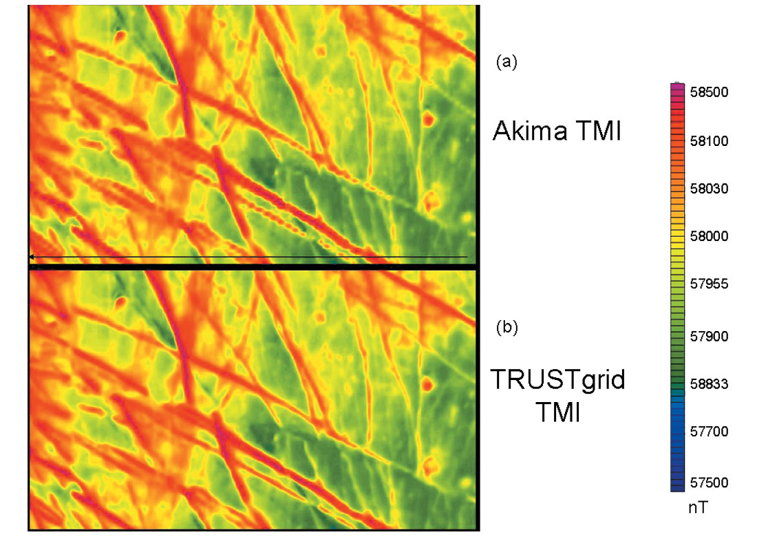
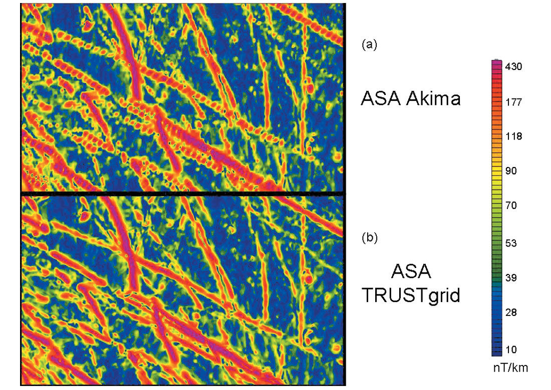
The advantage of using the TRUST grids for generating derivative maps is evident when comparing images derived from untrended grids with the images derived from trended grids generated using the TRUST grid process. Figure 2a shows the total magnetic field using an Akima bi-directional spline (Akima 1970, 1972). The traverse line direction is horizontal in this case (black arrow). Some features show the boudinage artifacts, particularly those in the middle of the bottom of Figure 2a. The grid generated using the new TRUST gridding process is shown in Figure 2b. There are very few boudinage artifacts on Figure 2b. The ASA images derived from Figure 2a and 2b are shown in Fuguro 3a and 3b respectively. The derivative enhancement applied to the untrended data makes the boudinage artifacts even more apparent. In fact, on Figure 3a, there are about 300 discrete features apparent and most of which are artifacts of the gridding process. The large number of these features can be distracting and make interpretation of the subsurface geology more difficult. The ASA derived from the TRUST gridded image is shown on Figure 3b. In this case, there are very few artifacts associated with the gridding process, so interpretation will be easier. Some interpreters use the width of the ASA features to estimate the depth to a contact model (Roest, et al., 1992). The widths on Figure 3b, better reflect the actual width, so the interpretations from this data will be more accurate.

Comparison with other methods for trending data

Reford (2006) compares a number of different methods for trending data using data published by the Geological Survey of Canada (2001). In order to enhance the narrow features, he applies two passes of a 3 by 3 Hanning filter and then subtracted this filtered grid from the original data. The untrended image generated using a bicubic spline and enhanced in this manner is shown on Figure 4. The traverse direction is shown with the white arrow at the top right of the figure. Boudinage artifacts are evident on the image particularly on the top left of the image.

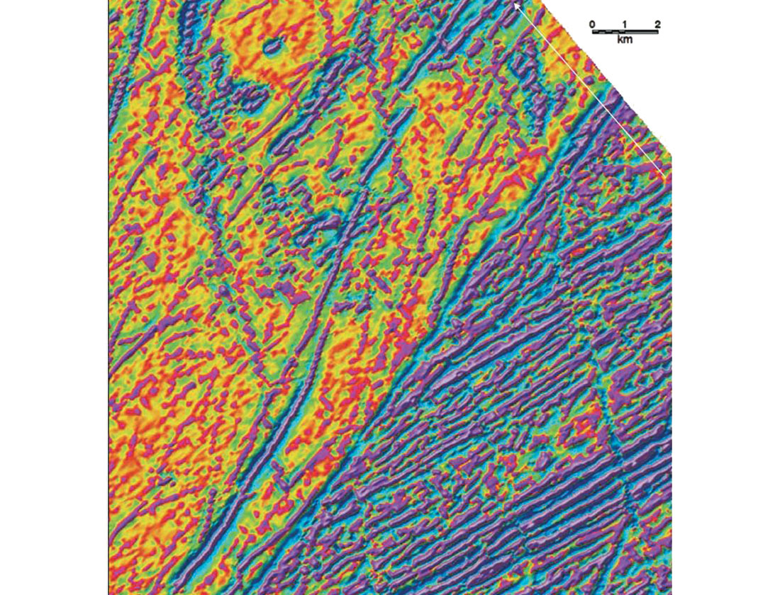
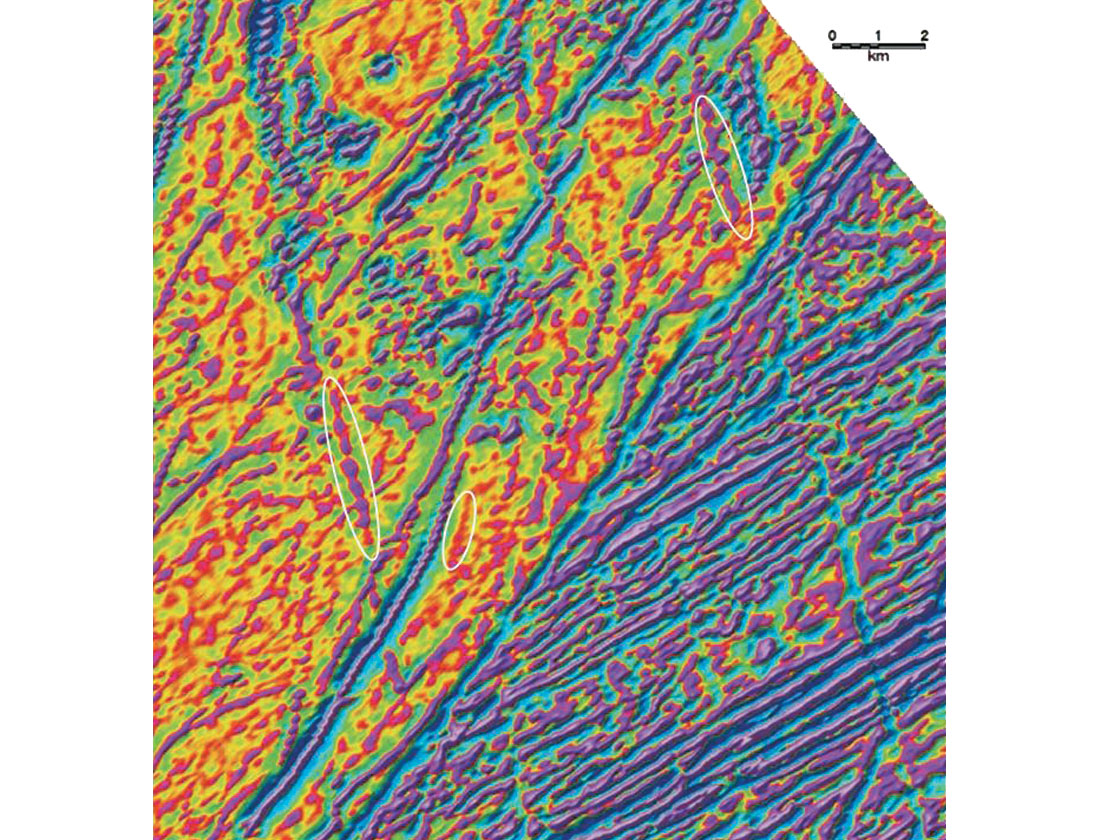
Figure 5 shows the data trended using Nelson’s (1994) method and bicubic spline interpolation. This method uses the measured horizontal gradients to aid in trending. The boudinage artifacts are still evident in the top left of the figure, but there has been some improvement, particularly on the features highlighted with a white ellipse.

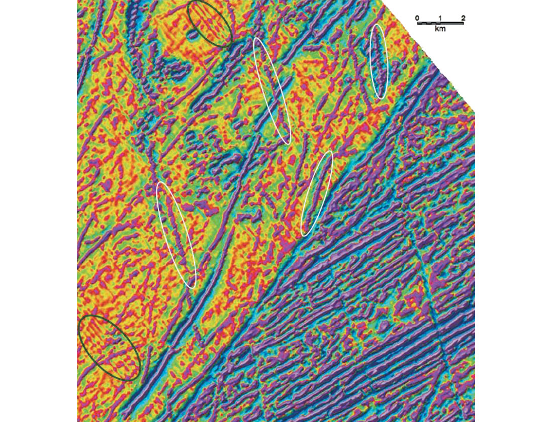
Hardwick’s (1999) method (which also uses measured gradients) provides further improvement of these and other features (highlighted in white on Figure 6), however, it also adds artifacts along the traverse lines (highlighted in green). These artifacts are not necessarily a weakness of the method, but might be removed if the measured lateral gradient data used to generate the image were more carefully levelled. Unfortunately this levelling procedure can be a laborious process.

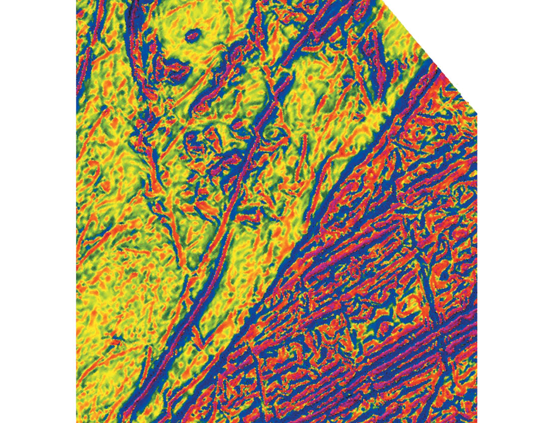
The data has also been interpolated using the TRUST gridding process. The image enhanced to show the narrow features in a manner similar to the Hanning residual used by Reford is shown on Figure 7. Unfortunately, the colour palette is different, so the images do not provide a direct comparison. However, it is possible to see that the features highlighted previously have all been well trended, as have the features in the top left of the image.

Conclusions

The TRUST gridding process generates grids that enhance narrow features trending at angles which are oblique to the traverse lines. An improvement to the algorithm ensures that artifacts along the flight line are not evident when calculating derivatives from the gridded data.

Compared with the untrended grids, the TRUST grids images show fewer artifacts, both on the total field images and on derivative maps such as the analytic-signal amplitude. When the TRUST grids are compared with other methods for trending data, they show better trending and fewer artifacts. This will mean that the maps will be easier to use for interpreting the subsurface geology and any quantitative information derived from the maps will be more accurate.