Imaging SAGD steam chambers: traditional ERT vs broadband electromagnetic methods

The Athabasca oil sands, located in Northern Alberta, Canada, are one of the largest oil reserves in the world. Over the last 30 years, industry has developed the Steam Assisted Gravity Drainage (SAGD) method to extract heavy oil that is too viscous to be extracted using conventional methods and is too deep for surface mining processes. SAGD uses a pair of horizontal wells to heat and extract the heavy oil. Steam is injected into the top well, which heats the oil and makes it less viscous. The mobile oil flows to the bottom where it is collected and pumped to the surface by the lower horizontal well. Heterogeneity within the reservoir can prevent the steam from flowing as expected, and thus limit the amount of oil heated and produced. Monitoring the steamed volume over time helps to identify problematic areas and also reduce the amount of water resources needed. Current monitoring procedures rely heavily on seismic imaging methods (Nakayama et al, 2010; Zhang et al, 2005). While successful in many cases, 4D seismic is expensive, may not be directly sensitive to the steam chamber itself due to minimal change in petro-elastic parameters, and can only be collected during the winter months when the ground is frozen. The steaming process also changes the electrical resistivity, where the amount of change depends on many factors, such as the formation itself, steam salinity, and steam temperature (Mansure et al, 1993). When the change is significant, electric and electromagnetic (EM) surveys may be able to detect the steam chamber. Instrumentation, to carry out the geophysical surveys, can be installed as permanent systems to collect data year-round and allow time-lapse images to be obtained. Tøndel et al (2014) conducted an electrical resistivity tomography (ERT) survey using two borehole observation wells and mapped the resistivity change due to steam chamber growth. Currently, the cross-well ERT, coupled with 2D inversions, is the general state-of-practise. In this paper, we investigate a wider class of EM surveys and show the enhanced images that can be obtained by using broadband data and carrying out inversions in 3D. To compare the efficacy of the different surveys, we introduce a representative geologic model for the Athabasca oil sands. We show that broadband EM surveys with a moderate number of transmitters and receivers have the potential to answer some questions about the location of the steam and that this potential should be further followed up with petrophysical studies and a trial field experiment.

Synthetic model

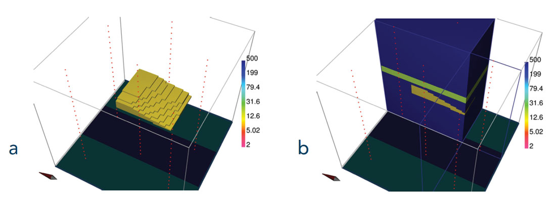
To test the feasibility of EM methods, a synthetic model was generated. The Athabasca oil sands range in depth from the surface to a maximum of 400 m (Hinkle and Batzle, 2006). The strata can be simplified into a few distinct layers: the Quaternary containing glacial tills, the Clearwater shale cap rock, the McMurray oil sands reservoir, and the Devonian limestone unit. Table 1 shows typical thicknesses and resistivity values for each of these units. Using values from within these ranges, we design a synthetic model, shown in Figure 1. The heavy oil reservoir begins 200 m below the surface and has a thickness of 60 m. The oil reservoir and surrounding units are assigned a resistivity of 400 Ωm while the cap rock has a resistivity of 17 Ωm. The cap rock is essential for SAGD processes because it prevents steam from rising to the surface. Here, it is modeled as a 25 m thick layer. The irregular steam chamber in the bitumen reservoir is 150 m by 200 m in the easting and northing directions and its thickness varies from 5 to 50 m. The upper surface of the steam chamber is 10 m beneath the undersurface of the cap rock. The oil reservoir resistivity is expected to decrease due to steaming (Mansure et al, 1993). The extent of the change depends on the reservoir parameters such as lithology, steam temperature, and steam salinity (Butler, 1995). For this paper, based upon previous literature, we assume conservatively that the bulk resistivity of the steam chamber is 10 Ωm.

TABLE

DC resistivity

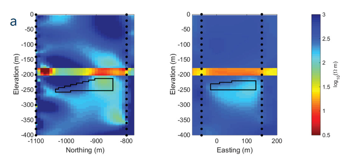
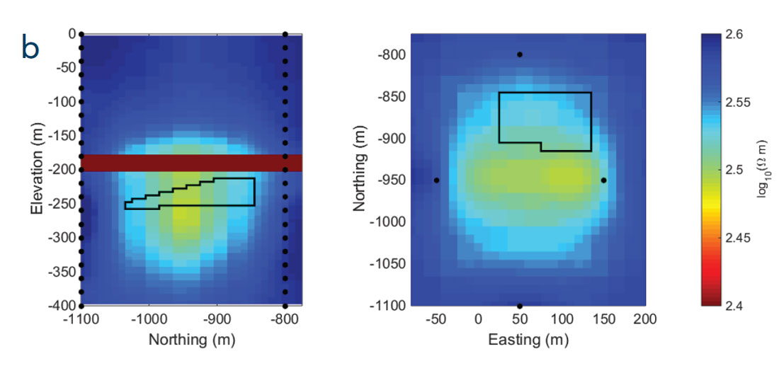
Cross-well DC resistivity (ERT) surveys are standard for fluid monitoring (e.g., Daily et al (1992), LaBrecque et al (1996), Tøndel et al (2014)). We design such a survey using four boreholes that straddle the location of the steam chamber, as shown in Figure 2a. The boreholes are spaced 200 and 300 m apart, which is a realistic distance based on locations of observation wells for SAGD operations (e.g., Zhang et al (2007)). Using this configuration, we forward model the ERT data in 3D. To simulate usual practice, we invert each pair of cross-well data using a 2D inversion algorithm (Oldenburg and Li, 1994). The final models, shown in Figure 3a, are contaminated with substantial artifacts. As a next step, we invert the two sets of cross-well data simultaneously in three dimensions (Haber et al, 2012). This resolves the artifacts and produces a smooth, confined body (Figure 3b). However, the steam chamber appears as a blurred, smeared-out image with a resistivity that is far greater than the true value.

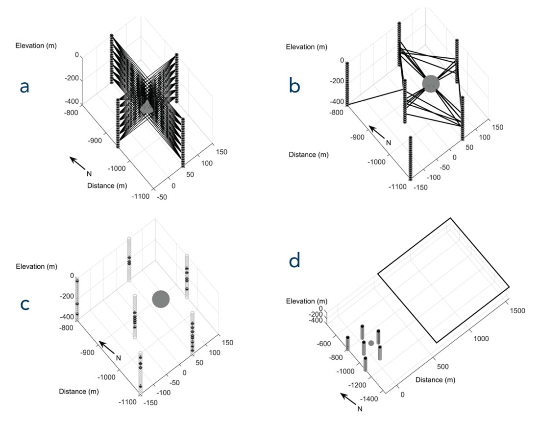
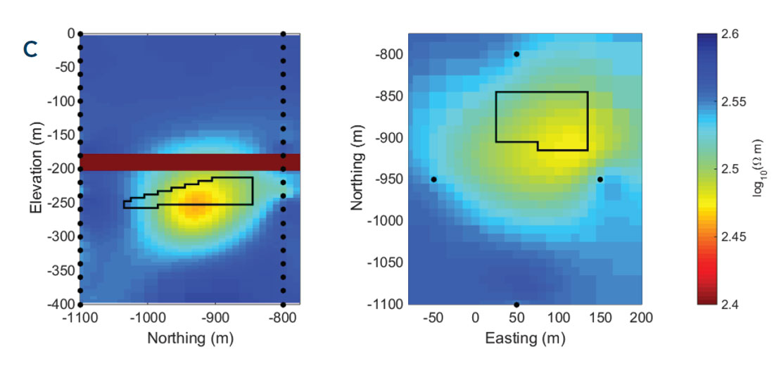
To increase the resolution, the survey was re-designed to better excite the steam chamber in three dimensions. Our approach uses anomalous secondary currents of a confined body to select current electrode pairs that will excite the steam chamber in multiple directions (Devriese and Oldenburg, 2014). The re-designed survey, with 24 current electrode pairs with 124 potential measurements for each pair, is shown in Figure 2b. We forward modelled and inverted the DC resistivity data in 3D (Figure 3c). The image of the steam chamber has improved in both shape and resistivity compared to Figure 3b. This indicates that the additional information from the 3D survey helps to constrain the model. Unfortunately, this model does still not provide enough information to confidently identify the anomaly as a regular or irregular steam chamber. An additional, and realizable, improvement can be made if the experiment is carried out as part of a time-lapse survey where an initial survey is conducted to reveal the background resistivity and a subsequent survey is conducted after steam injection. To simulate this, we carry out another inversion after specifying that the background, including the low resistivity cap rock, is known. Thus, only cells within the 60 meter thick bitumen layer are allowed to change in the inversion. The recovered image is shown in Figure 3d. The result has improved, especially in the recovered resistivity, but we can obtain better results by using electromagnetic methods.

Electromagnetic methods

DC resistivity is an electromagnetic experiment done at one frequency: f = 0 Hz. Unlike DC resistivity, electromagnetic surveys are conducted at multiple frequencies, or use time-domain waveforms. This should provide better results because each frequency samples the earth differently. A fundamentally important concept is skin depth. Skin depth is the distance (d in metres) that a wave propapropagates before attenuating by a factor of 1/e and is generalized as , where ρ is the background resistivity (Ωm) and f is the frequency (Hz). The distances from the transmitter to which observations are sensitive are inversely proportional to the frequency.

We now use the same current electrode pairs as the DC example at seven frequencies ranging from 1 to 10,000 Hz. The secondary currents induced in the steam chamber have different amplitudes and phases for each frequency and thus, observed data encode different information about the chamber. Modelling these data requires solving the full Maxwell’s equations for which we use a finite volume technique (Haber et al, 2004).

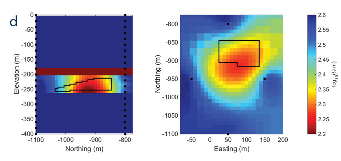
The data, which now include both electric and magnetic fields, are contaminated with 2% Gaussian noise and inverted in 3D. The initial model contains the background with the cap rock layer. However, only the resistivity within the bitumen layer is allowed to change during the inversion. The recovered model (Figure 3e) is far superior to any of the inversions that use only the DC data. The irregularity of the steam chamber is imaged; it becomes progressively thinner towards the south-west and the depth to the top of the steam increases. Furthermore, the chamber manifests itself as a substantial conductor, which contrasts the muted dynamic range of the resistivity recovered with DC resistivity (Figures 3c and 3d). Overall, by using multiple frequencies and designing a 3D survey, we obtain important information about the existence, location, and detail of the steam chamber.

Additional survey geometries and considerations

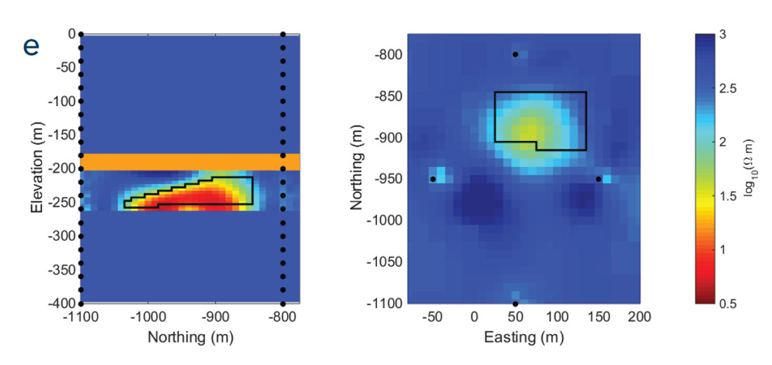
In the previous examples, we demonstrated that EM surveys are capable of imaging SAGD steam chambers. A cross-well survey was employed in which the transmitters were grounded electrodes and the receivers measured the electric potentials, electric fields, and/ or magnetic fields. The transmitter currents were harmonic and the measured data included the primary fields as well as the desired secondary fields from the target. However, there are many other EM survey designs that could be implemented. The choice of which survey to use depends upon many factors that include acquisition costs, field logistics, resolving power of the survey, and the ability for processed data from the survey to provide an answer to the posed question. For example, it may be desirable to use cost-effective magnetic sources rather than electric sources in a borehole. We use our survey design approach to delineate locations for 29 vertical magnetic dipole transmitters within the 6 borehole used in the previous example (Figure 2c). Noise-contaminated electric and magnetic fields, measured at 125 receivers within the boreholes for the same 7 discrete frequencies as before are inverted. The model (shown in Figure 3f) recovers the essential shape and the resistivity of the steam chamber.

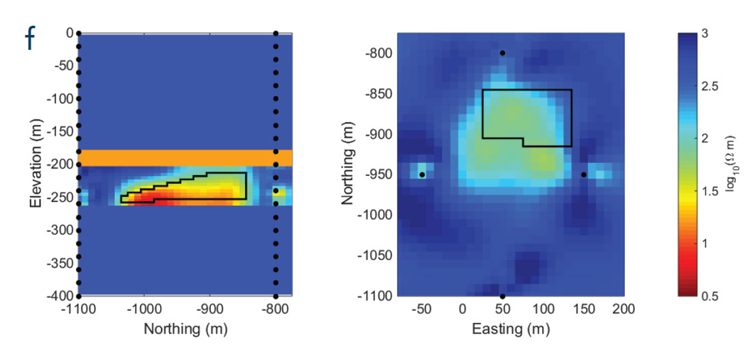
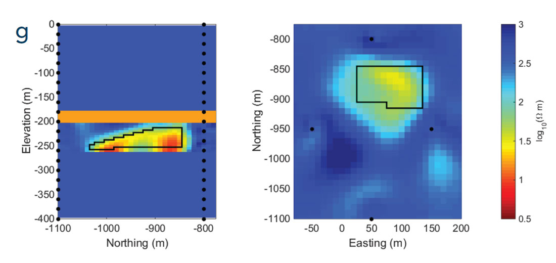
Survey costs undoubtedly would be further reduced for transmitter and receiver combinations located at the surface. For the geologic configuration explored here that appears to be difficult, especially if grounded sources are used. The conductive cap rock is the main obstacle because it channels currents out of the region before they reach the steam chamber. Nevertheless, the combination of surface and borehole instrumentation may be effective. This situation drives our next example, using the same boreholes with 126 receivers, but the transmitter is a 1 km by 1 km loop at the surface (Figure 2d); this is similar to previous case histories (e.g., Mutton, 1987; Spies, 1996). The same 7 discrete frequencies are used and electric and magnetic data are forward modeled and corrupted with noise. These data are inverted using the same constrained model. The recovered model is shown in Figure 3g, and the results are similar to the other two EM inversions where the shape and the resistivity of the irregular steam chamber are recovered.

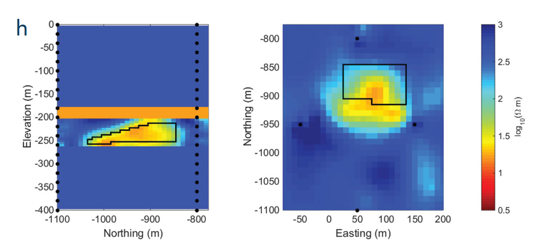
As a complement to the frequency-domain experiments considered thus far, we also explore the use of time-domain EM. We repeat the example using the surface loop and borehole receivers (Figure 2d), but forward model both the magnetic field and its time-derivative based on a step-off waveform (Oldenburg et al, 2013). Data are measured at 11 off-time time channels ranging between 4 and 60 μs. The inversion of these data yields the recovered model presented in Figure 3h. The result is similar to the frequency-domain inversion (Figure 3g) with good recovery of both the shape and resistivity of the irregular steam chamber.

To summarize, the steam chamber was adequately recovered in all four EM examples but the results were slightly different. Sources within the boreholes are ideal because they can be used to excite the anomalous area in all three dimensions. Restricting the survey to surface transmitters limits the excitation directions and hence directions of the anomalous currents; this limits the amount of information that can be obtained about the subsurface. Nevertheless, the latter two examples showed that for a surface transmitter and borehole receivers, both the frequency- and time-domain methods can provide informative images.

Conclusions

We have investigated the potential of electromagnetic surveys for imaging steam chambers in SAGD. A geologically reasonable example provided the basis for our experimental study. We showed that carrying out a single cross-well DC resistivity survey involving 2 boreholes resulted in artifacts if the inversion is carried out in 2D. Inversion of these data in 3D resolved the artifacts but the recovered model lacked resolution. Therefore, both data acquisition and inversion in 3D are necessary. Unfortunately, there are an overwhelming number of survey design variables that include: transmitter geometries and types, the choice of harmonic or step-off transmitter waveforms, the types of measured data (e.g., using some or all components of the electric and magnetic field), and receiver locations. In our work, we limited data acquisition to realistic observation well locations at a potential field site and we limited transmitter types to those that are readily available. The best images were obtained using borehole transmitters and receivers operating either in the frequency domain or time domain. However, our findings suggest that cheaper options that involve surface loop transmitters and borehole receivers may yield valuable insight about the steam chamber. The resistivity values used in this paper were based on literature that is specific to the Athabasca oil sands, but the methodology is transferable to other heavy oil reservoirs. The resistivities in those settings will depend upon numerous factors, and determining them will require extensive in-situ and laboratory petrophysical analyses. Nevertheless, our work shows that if the steam is conductive with respect to the background bitumen layer, then the steam chamber can be imaged using realizable surveys with frequency-domain or time-domain electromagnetic systems. This aids monitoring of the steam chamber growth to help optimize oil production in SAGD projects.

Acknowledgements

We would like to thank Martyn Unsworth and Mostafa Naghizadeh for the invitation to submit this article to CSEG RECORDER.