Networked systems require the consideration of interactions between component parts as well as the parts themselves in understanding the properties of the system. In the case of hydraulic fracturing, the process can be regarded as the spread of a fractured state through an initially unfractured network of rock elements. In this study, we implement a spreading model in networks to evaluate the dynamics of the hydraulic fracturing process in various rock types defined by their relative proportions of quartz and clay. The corresponding results demonstrate that the energy required to initiate fracture propagation increases with increasing clay content. Furthermore, the areal extent of fracture propagation increases with increasing quartz content. These results are in qualitative agreement with empirical observations. Additionally, the velocity and acceleration of the fracture propagation front exhibit a shape that is typical for a relaxation phenomenon.
Introduction
Many macroscopic phenomena manifest as the result of a network of interacting agents and often exhibit dynamics that are reciprocal to its network structure. These network interactions govern phenomena ranging from collective behavior in schooling fish (Figure 1) to the spread of viruses in human networks. In these networked systems, the interactions between component parts are just as important as the parts themselves in defining the properties of the system (Motter and Albert, 2012). In addition, it is widely accepted that macroscopic phenomena do not depend on the microscopic details of the process, as in effective field theories that are applicable at some chosen length scale and ignores the substructure and degrees of freedom at shorter distances. Therefore, the description of seemingly complex phenomena can be greatly reduced in complexity by application of the above paradigms. In this study, we apply these concepts to hydraulic fracturing to investigate the dynamical process under which hydraulically induced fractures propagate in various rock types. These simplifications allow us to discard the complex fluid flow and fracture mechanics in modeling the dynamic response of hydraulic fracturing (e.g., Lutz, 1991). It should be noted that the simplified approach presented here only provides qualitative descriptions and lacks the rigor in understanding the phenomenon at a fundamental level. It does however provide an alternative conceptual view of the problem.

Many observations concerning fracture propagation in so-called brittle or ductile rocks have been well established with the aid of empirical data, where brittleness is often associated with higher quartz content and a corresponding low Poisson’s ratio. For example, engineering data such as the instantaneous shut in pressure (ISIP), which provides an indication for the stresses that must be overcome for fracture propagation, was found to correlate with Poisson’s ratio (e.g., Maxwell et al., 2011). Additionally, it is generally observed that fractures propagate further in brittle rocks while propagation is more localized in ductile rocks, as suggested by microseismic event locations. In the following, we implement a simple network spreading model in an attempt to model the dynamics of the hydraulic fracturing process and evaluate the corresponding fracture propagation response for various rock types.
Fracture spreading model
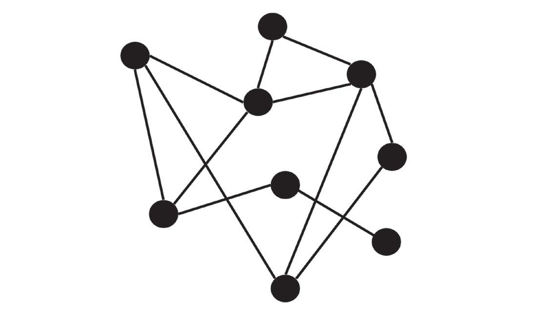
Here, we adopt the abstraction of a network to represent a rock mass with interacting elements, where the network consists of a set of nodes connected by lines or edges as illustrated in Figure 2. The network is a purely theoretical object but provides an extremely useful representation of complex systems with interacting components (Newman, 2008).
To investigate the dynamics of fracture propagation through a network of rock elements, we implement a spreading model proposed by Watts (2002) for the description of global (e.g., very large) cascades on random networks. In the model, a binary decision with externalities (Schelling, 1973) is considered. For a given network, each individual in the population, represented by a node, must decide between two alternative actions, where their decisions are based solely on the actions of other members in the population. Examples of such phenomena include everyday experiences such as deciding on which restaurant to visit. Because we often have limited information, we rely on the recommendation of others in our social network to aid in the decision making process (Figure 3). Further, these phenomena often exhibit a threshold nature whereby a specific number of connected nodes in a given state can trigger an individual node to alter its state. For example, if one favors Italian cuisine, it would require fewer recommendations to visit a certain Italian restaurant. Furthermore, large spreading events are occasionally observed where a small number of activated nodes trigger a cascade through the network. For the restaurant example, a previously undiscovered restaurant could gain popularity very quickly given the right conditions for the spread of information through a social network.

In the case of hydraulic fracturing, the process can be regarded as the spread of a fractured state through a network of initially unfractured rock elements. For the model specification, we consider a population where an individual agent observes the states (0 for unfractured or 1 for fractured) of its connected neighbors, where the range of connections is known as the degree, and if a certain threshold fraction, defined on the unit interval, is achieved, it adopts state 1, else it remains in state 0. To initiate the system, a set of seed nodes are placed in the network and the process is subsequently iterated through a series of time steps. A successful hydraulic fracture treatment is then defined by a cascade event, where if a cascade is triggered, state 1 spreads throughout the network and if a cascade is not triggered, the network remains in its initial state. In the following, we define the threshold and degree as required by the spreading model.
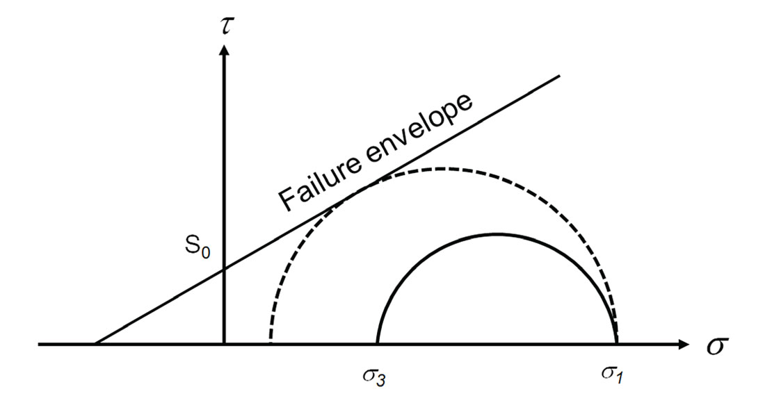
To calculate the threshold, we implement the uniaxial strain condition for loading of an elastic solid given by

where ν is the Poisson’s ratio and σ1 and σ3 are the maximum and minimum principle stress magnitudes respectively. For a given value of σ1, a lower value of σ3 can be achieved through lowering the value of ν. According to the Mohr-Coulomb failure criterion, this results in a larger Mohr circle and hence is more easily fractured as illustrated in Figure 4. Since the quantity ν/(1-ν) is defined on the unit interval for all values of ν between 0 and 0.5, it can readily be used for the threshold condition. Therefore, a material with a lower Poisson’s ratio is more easily fractured and thus requires less influence to achieve failure.
To calculate the degree, we consider how information is transferred in an elastic solid. Upon the application of a stress, particle motion is excited through strain waves that propagate throughout the medium. Therefore, we associate the transfer of information regarding the state of stress through the mechanics of wave propagation. The wave equation can then be used to evaluate how energy propagates in an elastic solid and provide an indication for the range of connected nodes. In a 3D homogeneous medium, the Green’s function for the scalar wave equation is given by

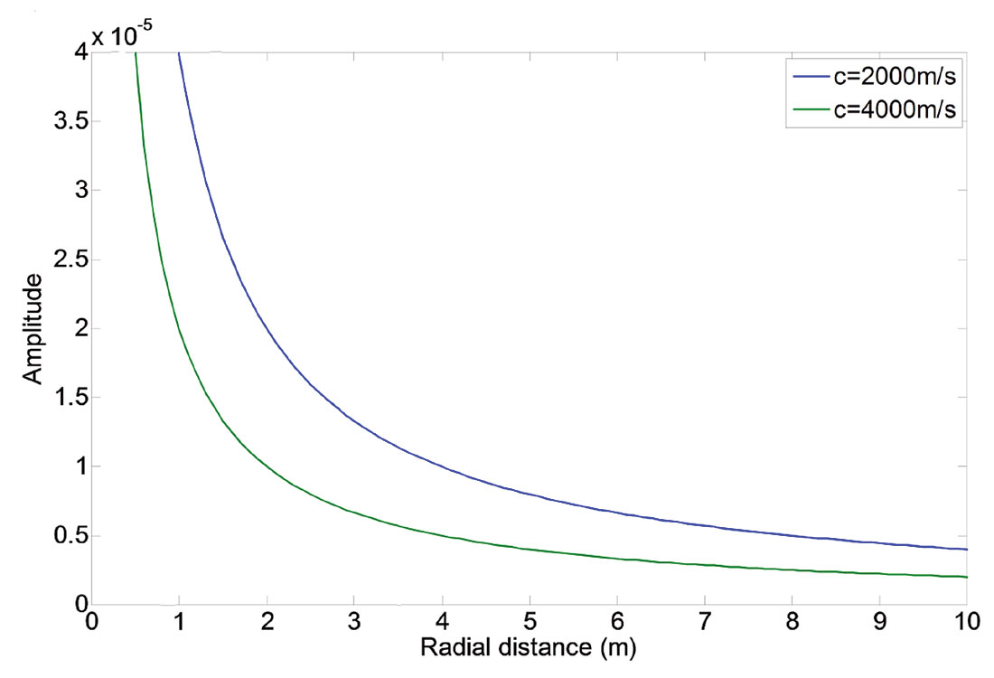
where c is the P-wave velocity, t is time, r is the radial distance from the source location and δ represents an impulse function. According to equation 2, the rate at which the amplitude decays is inversely proportional to r and is scaled by the inverse of the P-wave velocity. Therefore, a material with a higher value of P-wave velocity experiences more amplitude decay at a given radial distance, r, from the source point (Figure 5) and results in a more localized connectivity.
Dynamical modeling
For the evaluation of the fracture propagation response in different rock types, we use the mean of the Hashin-Shtrikman bounds (1963) for a two-phase material consisting of varying mineral fractions of quartz and clay. With this approach, we avoid the ill-defined concept of brittleness which is not a fundamental property of an elastic solid.

Figure 6 shows the upper and lower bounds and mean for the P- and S-wave velocities and the corresponding threshold and degree for the two phase material. The elastic properties of the two mineral end members used in the computations are given in Table 1.
| Mineral | ρ (g/cc) | VP (km/s) | VS (km/s) |
| Table 1. Density (ρ) and P- (VP) and S-wave (VS) velocities used for the mineral end members (from Greenberg and Castagna, 1992). | |||
| Quartz | 2.65 | 6.05 | 4.09 |
| Clay | 2.66 | 4.32 | 2.54 |
To evaluate the dynamics of the hydraulic fracturing process, we solve the system numerically and analysis the corresponding results. The simulations were performed in 2D for each set of mineral fractions ranging from pure clay to pure quartz. As mentioned above, we attribute a successful hydraulic fracture treatment with a cascade event triggered by a specific number of initially active nodes. We are then interested in the number of seed nodes required to trigger a cascade and the evolution of the system through time. Figure 7 shows the propagation of the fracture front at various snapshots in time for rock models containing 10 and 70 percent quartz.
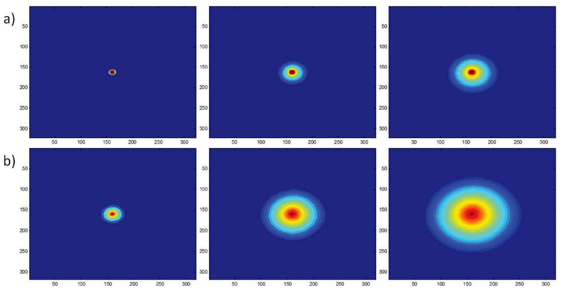
Figure 8a shows the phase diagram illustrating the cascade boundary. As the threshold is crossed from the no cascade to cascade region, a chain reaction is initiated and the fractured state will continue to propagate throughout the grid. This perpetual propagation response is the result of a grid consisting of only unfractured states and an implicit condition of unlimited energy input. In reality, fracture propagation could be interrupted by the interception of natural fractures (analogous to a control line to prevent the spread of wild fires) or a decrease in hydraulic pressure to a level that is below the threshold for fracture propagation. Figure 8b shows the stimulated area as a function of the volume of quartz. These results demonstrate that less effort is required to achieve a cascade (initiate fracture propagation) and a larger area is stimulated as the volume of quartz increases.
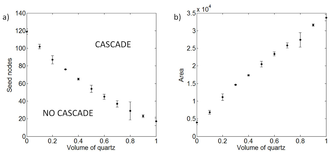
Figure 9 shows the ISIP gradients and microseismic event locations associated with the stimulation of three horizontal wells in the Montney shale of NE British Columbia, Canada. These results are overlaid on a map of Poisson’s ratio at the reservoir interval. The hot colors represent lower values of Poisson’s ratio and serves as a proxy for increasing quartz content and hence, brittleness. It should be noted that the Montney also contains a significant amount of carbonate; therefore an increase in the Poisson’s ratio could indicate a decrease in the quartz/clay or quartz/carbonate ratio. In Figure 9, lower values of the ISIP gradients are observed in more brittle rock. Additionally, the microseismic event locations indicate a larger stimulated area in more brittle rock. These observations are in qualitative agreement with the simulation results.
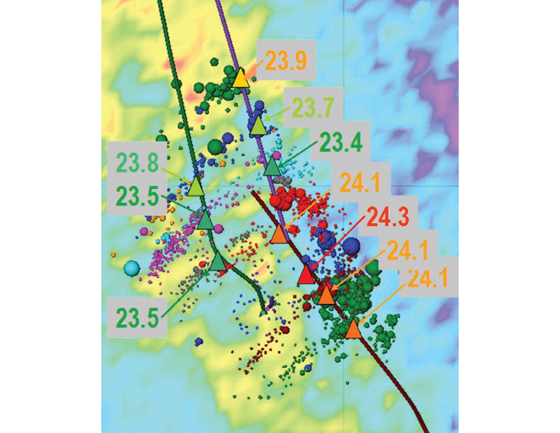
Figure 10a shows the number of activated nodes as a function of time. For comparison, Figure 10b shows the microseismic event (MSE) count as a function of time for various stages of a hydraulic fracture treatment in a shale gas reservoir. Note a similar character associated with the simulation results and field observations. Therefore, according to the proposed fracture spreading model, the variations in the observed MSE count between different stages can potentially be the result of variations in mineral fractions along the length of the lateral. In addition, note that the MSE count flattens out at certain instances in time. This response can potentially be explained by the interception of natural fractures where the fracture propagation front ceases and the process must once again be initiated.
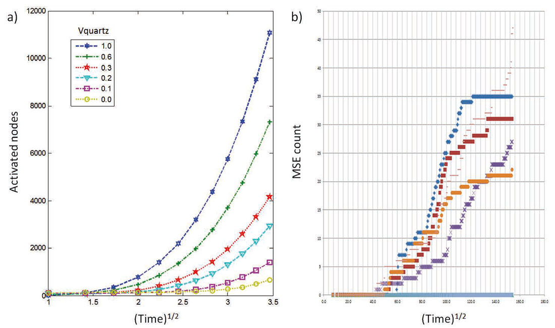
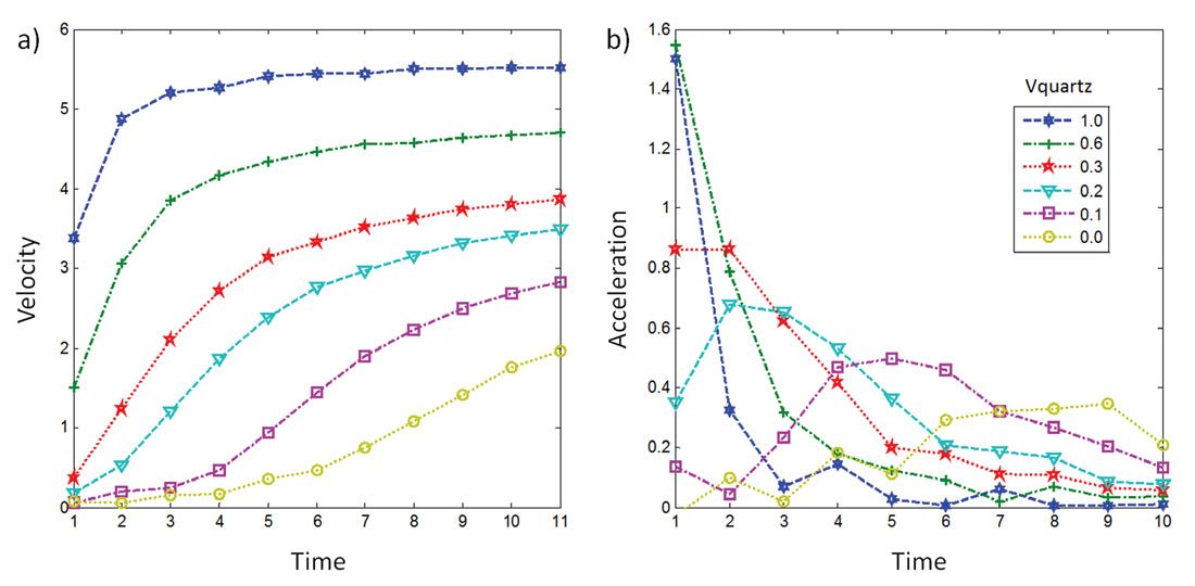
Figure 11 shows the velocity and acceleration of the fracture propagation front. The time variant response is likely due to interactions between component parts in the network of rock elements. Additionally, it is interesting to note that these curves exhibit a shape that is typical for a relaxation phenomenon. This suggests that the problem as formulated here can potentially be amendable to analytical treatment and modeled as a diffusion process.
Conclusions
The dynamics of the hydraulic fracturing process were evaluated through a spreading model for rock types consisting of varying mineral fractions of quartz and clay. This was performed to provide an alternative view of the mechanisms underlying the empirical observations documented by various authors concerning the fracture propagation response in so-called brittle and ductile rock. As the hydraulic fracturing process is a dynamical system consisting of numerous interacting rock elements, the interactions between component parts as well as the parts themselves must be considered in understanding the properties of the system. The simulation results were in qualitative agreement with empirical observations concerning the energy required to initiate fracture propagation and the stimulated area for varying mineral fractions of quartz and clay. Additionally, the velocity and acceleration of the fracture propagation front exhibit a time variant response that is likely due to interacting components within the network of rock elements.

Acknowledgements
I would like to thank Gary Margrave, Jeff Grossman, Bill Goodway and Marco Perez for discussions and an anonymous reviewer for helpful comments. Thanks also to Shawn Maxwell and Eric von Lunen for the use of their figures. The sponsors of the CREWES project are also acknowledged for their support.


Join the Conversation
Interested in starting, or contributing to a conversation about an article or issue of the RECORDER? Join our CSEG LinkedIn Group.
Share This Article