High-Resolution Crosswell Seismic Imaging Between Horizontal Wells

Introduction

Crosswell seismology is a proven high-resolution seismic imaging technology due to its ability to provide unusually high-frequencies conventionally unattainable by 3-D seismic. Numerous case studies have demonstrated its applicability as one of the most effective reservoir management tools. A recent report by Zhang et al. (2002), for instance, shows that very complex architectures of thin shale laminations encased within the thick bitumen-rich McMurray channel sands at a northern Alberta SAGD project site can be characterized confidently with the help of the very high resolving power of crosswell images.

But historically, crosswell seismic data had probably never been recorded in horizontal wellbores until recently. Several reasons are responsible for this fact. Firstly, oilfields had been developed through drilling mostly, if not all, vertical or deviated wells. It was not until about a decade ago that horizontal drilling became a common practice in field optimization. Even in new fields where horizontal drilling is adopted as a main development strategy, well spacing is commonly too large for crosswell seismic to be practically useful. Secondly, crosswell data processing and imaging techniques have become increasingly sophisticated, but only for the data obtained from a vertical-well (or similar) geometry.

Lastly and perhaps most importantly, no equipment (such as downhole sources and/or receivers) and deployment technology were robust enough and readily suitable for the use in a horizontal well environment. In general, conditions in a horizontal well are much more complicated than in a vertical well. In some special cases where customer-designed instruments are available, costs are often prohibitively high for seismic work within horizontal wells.

The month of August 2000, however, witnessed a landmark breakthrough when the novel idea of recording crosswell seismic data from horizontal wells was first attempted at EnCana Corporation’s Weyburn Field, located in southeastern Saskatchewan. The wells chosen for the survey are from the site of a massive miscible carbon dioxide (CO2) flood, planned to start a month later. A large volume of CO₂ gas in its super-critical phase would be injected into the carbonate reservoir from 19 injection patterns, most of them being horizontal wells. This pre-flood crosswell survey used a horizontal producer for downhole receivers and a horizontal injector for downhole source. Coiled tubing technology made deployment of the seismic instruments into horizontal wells possible and safe. High-quality borehole seismic data with a rich yet complicated wavefield were successfully acquired. Processing, although preliminary, of some of the data yielded a detailed picture of the reservoir.

Data Acquisition

The Weyburn reservoir, situated at an average depth of 1,450 metres, is composed of two layers of Mississippian-age hydrocarbon- saturated carbonate rocks: the upper layer (Midale Marly) is a dolostone 10-m thick or less, characterized by high porosity (20 ~ 37%) and low permeability, while the lower layer (Midale Vuggy), roughly 20 meters thick, is a limestone, less porous (2 ~ 15%), relatively permeable, and much more fractured than the Marly. Core and well log studies and 3-D seismic mapping have all shown a complicated reservoir nature of heterogeneity and anisotropic flow behavior. Seismically, the Marly dolomite unit is slow with an average velocity of 3,600 m/s, whereas the limestone in the Vuggy presents a higher velocity structure of 5,500 m/s. Immediately above the Marly, the reservoir is capped by impermeable tight rocks with high velocities. Over the past 40 years, water floods have swept largely the oil in the Vuggy zone, but left the Marly in a nearly virgin state.

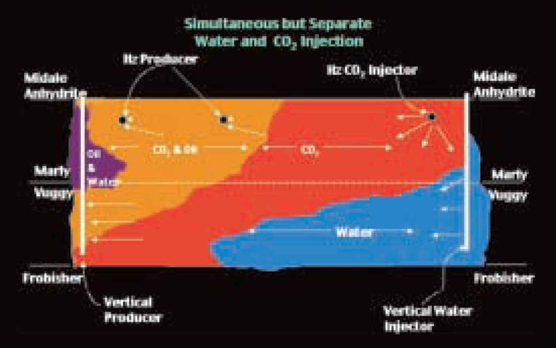
One of the major injection strategies called simultaneous but separate water and CO₂ injection (SSWG) is illustrated in Figure 1. In this scheme, CO₂ is continuously injected into the unswept Marly zone from horizontal wells, and should firstly migrate downward into the Vuggy zone, because of the significant differences in pressure and permeability between the two layers. The miscible CO₂ should displace the residual oil in the Vuggy. Subsequent water injection from vertical wells into the Vuggy will help pressure it up and force the CO₂ fluid to move upward. Also due to gravity override, the up-moving lighter CO₂ will help push the Marly oil. Oil from both zones will be produced by vertical as well as horizontal wells. Apparently, this exciting yet challenging engineering innovation implies a certain degree of uncertainty and hence makes seismic monitoring necessary.

The primary objective of our crosswell survey was to acquire high-resolution baseline seismic information for a comprehensive time-lapse monitoring program, which includes multi-component 4-D seismic, in this EOR project. The high-resolution data from the survey were believed to help better characterize, in the interwell space, the small-scale reservoir rock features, whose effects on CO₂ flow behavior may be of importance. The subsequent time-lapse surveys as planned would provide more detailed in-situ information about CO₂ front movements and interactions with reservoir features such as fractures. Our secondary objective was to integrate the crosswell information as a necessary part of cross-disciplinary, multi-resolution integration for dynamic monitoring of CO₂ flood and storage.

Two reasonably parallel horizontal wells from an SSWG pattern were used in our survey. A perspective view of their geometry is given in Figure 2. Both wells are located within the Marly zone and they are separated by between 250 to 270 meters. The source well indeed is one of the dual laterals of the injection well, cased all the way to the corner. On the other hand, the production well, in which the receivers were placed, was cased only in the vertical section but not around the corner, which gave rise to some difficulties when we deployed the receiver tool through it. The horizontal legs of both wells were completed as open holes with an extent of nearly 1,000 meters. They are nominally 7 inches wide I.D. in the open-hole sections. Notice that the direction of the wells runs against each other, resulting in unwanted limitations in lateral coverage of the data we recorded.

The strong velocity contrasts in the reservoir and its adjacent background rocks made design considerations of the survey critical for imaging the slow Marly layer. Standard ray tracing and finite-difference elastic modeling were performed (Majer et al., 2001). The modeling results revealed a few things valuable for survey planning and design. For example, the high-velocity layers on either side of the thin Marly layer control the first arrivals in the crosswell data. Because of large contrasts in velocity and enough spacing between wells, separation between the first arrivals (most likely refracted or head waves) and the coda of slower arrivals (propagating within the Marly) should be expected. Elastic-wave modeling also showed that the first arrivals should have low amplitude compared to later arrivals. The high amplitude coda subsequent to the first arrivals includes a direct wave, and perhaps guided wave modes, as well as their shear-wave counterparts. The guided wave modes appear to be of the highest amplitude, with definite dispersive characteristics.

Position control in a horizontal well environment is another prime concern for the survey design. In vertical wells, crosswell technology is well developed to place instruments exactly on depth using wireline technology. In long horizontal wells such as the subject case, there was no established deployment technology available. For this work, it was critical that not only absolute position be maintained, but that repeatability to within a half meter be maintained as well. This was necessary to ensure that time-lapse data changes due to positioning errors are relatively less than the expected time-lapse changes due to injection of CO₂.

Also of concern was coupling to the formations, especially if amplitude studies were to be performed. Other factors controlling the acquisition were the time allowed to do the survey, the overall cost, the size and length of instruments that could be placed in the wells, and safety issues (this is an H₂S site).

Based on our understanding from modeling, it was determined that equipment allowing for recording wide-band signals at a few meter spacing be used, in order to achieve the high frequency (over a kilohertz) content necessary to resolve the thin beds, and to provide a wide bandwidth for dispersion studies. Considerations were also given to the protection of wellbore integrity, avoiding the occurrence of getting the tools stuck in any hole. Many different options for field data acquisition and well operations were considered.

Coiled tubing deployment was eventually adopted to deploy the downhole equipment. A piezoelectric source from TomoSeis Inc. was selected. This source was modified to fit on the end of coiled tubing. To do this required protective spacers, and the source power cable run through the center of the tubing. This all had to be a sealed device, which created issues if the tool could not be pushed far enough, i.e., in most coiled tubing jobs, fluid can be injected out of the end if obstructions are encountered. This was not the case here for both the source and receiver string.

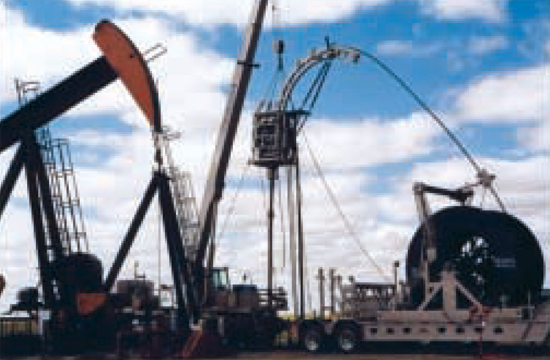
For receivers, we had considered the choice between three-component geophones and hydrophones. Ideally we would have liked to have three-component recording, but factors on wellbore safety and unknown limits on pushing the string limited us. We chose to deploy an oil-filled coiled tubing that had a total of 48 levels of hydrophones at 15 meter spacing. This unique coiled tubing deployment configuration was constructed by OYO Geospace Inc. and TriCan Well Service Ltd. The result was a dedicated coil tubing, with hydrophones inside, for this and other projects. Figure 3 shows TriCan’s coiled tubing unit injecting the 48-level hydrophone string into the horizontal producer.

During acquisition, the piezoelectric source was placed in the injection well as far as possible. Several repeat runs were done to ensure that we had confidence in the placement. The final location was at nearly 2,200 meters measured distance. The receiver coiled tubing was then pushed as far down the production well as possible. Due to the uncased section around the corner, this push was very difficult and it took several days to get final placement. The 48-level hydrophones were at 15 meter spacing, residing within the coiled tubing.

The source generated a sweep of 200 to 2,000 Hertz every 3 meters. After the source was pulled along the horizontal section of the well, it was pushed back to its starting position for another run. The receiver string was then pulled three meters and the source positions were reoccupied. This was done five times in total so that a complete crosswell survey at three-meter spacing was acquired. In order to check source repeatability on the last run, the source sweep was repeated while the hydrophones were kept in place.

Except for some difficulties at the beginning in placing the hydrophone array into the receiver well, the field job afterwards became quite smooth. A total of 56,000 crosswell seismic traces were recorded, with good quality and a wider-than-expected bandwidth of 200 ~ 1,700 Hz. The entire recording was done in less than 25 hours.

Results

Figure 4 shows a common receiver gather of the raw data collected from Weyburn. The corresponding depth of the receiver is at 1,920 m. The source depth ranges from 1,450 m to 2,165 m, sampled at 3 m. We were encouraged by the richness of the wavefield contained in the raw data. Since the wavefield corresponds to an unusual geometry resulting from the use of horizontal wells, identifying various wave modes is not as straightforward. The following is one possible version of the interpretation of the data.

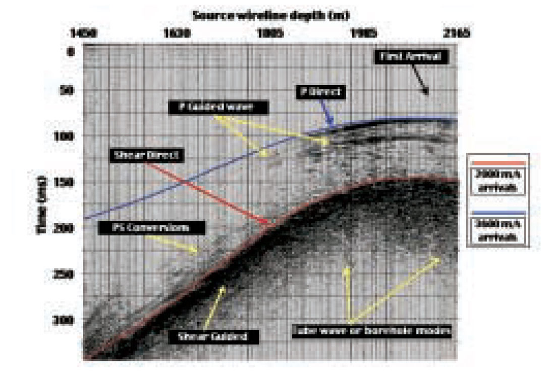
Ray-tracing modeling was used to help identify those seemingly obvious events in the data. We first tried to determine the nature of the strong event that appears around 80 ms in time. We superimposed on the data the calculated traveltimes (blue line) for a compressional direct wave traveling at a constant velocity of 3,600 m/s (which is Marly’s average velocity) and found that the tracing curve fits the arrival times and moveout curve of that event very well. We did the same thing for this similar event in other common receiver gathers and the fitting approach was found to work as well. Therefore, we believed that this event was a direct P-wave propagating directly within the Marly zone at its interval velocity, from the source to the receiver.

Next, we tried to fit the strongest event occurring at 145 ms with a moveout curve (red line) calculated at a shear velocity of 2,000 m/s, assuming a Vp/Vs ratio of 1.8, which is the average found for the reservoir zone from dipole sonic logs in this area. Evidently, the calculated times track closely the moveout of this event. So it was determined to be a direct S-wave traveling within the Marly interval.

With both direct P- and S-waves identified, it was then relatively easy to interpret those waves following them. The dispersive characteristics of these later events meet the description for guided waves, as revealed in our elastic wave modeling. They were thus interpreted as guided P- and S-waves, respectively. Apparently the data are quite ringy, making it very difficult to distinguish the guided modes from the direct arrivals in the process of event picking.

First arrivals in this gather were found having a very weak amplitude. They arrived around 60 ms and later, proceeding the direct P-wave and guided waves, matching our modeling predictions. The first arrivals in some other common receiver gathers appear to be stronger in amplitude. But overall they were very difficult to pick. In addition, several other wave modes, such as PS converted waves and tube waves, were also identified.

The event identified as direct P-wave was difficult to pick for processing for several reasons. Usually crosswell processing can exploit a variety of sorting domains for arrival discrimination and picking (Li and Stewart, 1996a and b). However, in our case, gathering the data into different domains did not provide particular advantages, due to the unusual geometry. The ringy nature of the data plus some difficulties with receiver well depth control made it difficult to correlate arrivals across gathers. Furthermore, as evident in Figure 4, the amplitude of the direct arrivals can vary greatly across the surveyed wireline depth range. These events could have been picked for all gathers if a special picking program was devised. However, to meet the preset processing deadline to make the final images available, only 30% of the traces collected were manually picked and used in inversion.

Utilizing these picks, TomoSeis performed tomographic inversion with a modified version of the 3-D crosswell regularized nonlinear inversion technique (Washbourne and Bube, 1998). Unlike “first-arrival” tomography, a method based on wavetracing that more accurately modeled the slower direct waves (Bube and Washbourne, 2001) was employed. This new method enabled one to estimate finite-frequency seismic propagation paths and arrival times that should be more consistent with our direct arrival picks.

The resulting velocity tomogram for the P-wave direct arrival is shown in Figure 5. In the interwell space, two high-velocity anomalies were identified ranging from 3,600 to 4,200 m/s, within a relatively lower velocity background of 3,400 m/s. Based on the velocity-porosity relationship available in the study area, we interpreted these anomalies as two continuous areas of relatively low porosity, compared with the surrounding higher porosity areas represented by lower velocities. We also noticed the presence of some linear stripes in the tomogram, which were thought to be possibly related to some acquisition/processing artifacts.

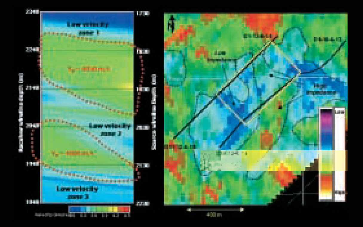
A small map of P-wave acoustic impedance, extracted from a surface multicomponent 3-D survey, is also shown in Figure 5 (right side), with the crosswell image area highlighted. It is interesting to note that the two higher-velocity anomalies identified on the tomogram correlate remarkably well to the two corresponding areas in the 3-D map of relatively high impedance values. Surrounding them are lower impedances, which match low velocities on the tomogram. Obviously, the correlation in the interwell region between the tomogram and the impedance map is great. However, the anomalously higher impedance zones in the 3-D map are not as sharply defined as in the tomogram, perhaps because of limited spatial resolution inherent in the 3-D survey. We believe that the crosswell profile should have the advantage over the 3-D seismic to image more fine-scale heterogeneities in that space with better resolution and higher fidelity, regardless of its limitation in dimension.

Conclusions and Discussion

A leading-edge crosswell seismic survey, recorded between two deep horizontal wells each with a lateral length exceeding 1,000 meters, was successfully completed at the Weyburn Field. This unprecedented survey yielded over 56,000 traces of high quality data. The recorded data exhibited a wavefield rich in many useful wave modes, mostly matching the ray-tracing and elastic-wave modeling results. High frequencies (200 ~ 1700 Hz) contained in the data made imaging fine-scale hetrogeneities in reservoir zones possible. Test-mode processing of the data and, specifically, tomographic velocity inversion based only on direct P-wave traveltimes generated an interpretable tomogram between two horizontal wells, never seen before in this world. The high-resolution crosswell tomogram detected and defined the seismic anomalies more accurately than the 3-D seismic impedance map with lower spatial resolution.

Conditions in horizontal wells are typically complicated. High entry angles, various engineering equipment emplaced inside the well (production tubing, packers, etc.) and tools and “garbage” unconsciously lost or forgotten, open-hole completion, varying wall size and depth variations along the horizontal trajectories, often hazardous formation fluids (such as H2S, and CO2), and so on, are commonly encountered in horizontal wells, and many of them were found to exist in the two wells we used for this survey. These conditions will make it difficult and sometimes impossible to access the wells for seismic work.

Careful planning, survey design, and modeling are all important. Employing proper equipment is essential. In our case, applying coiled tubing technology, although expensive, to deploy the downhole seismic equipment into the long horizontal legs, proved to offer much safety, flexibility, and ease of handling, all of which was highly desired for our survey. The specially-designed 48-level hydrophone system (injected inside the coiled tubing), long enough, and the powerful piezoelectric downhole source, able to be charged quickly enough for each fire, allowed the survey to sample the space more frequently, and to help us accomplish the objectives in a cost effective manner and within a production-constrained time window. Processing of crosswell data from horizontal wells is a tough task, since it is a completely new idea. Early processing efforts sofar indicate an excellent opportunity for making a full use of compressional-, shear-, and guided-waves in imaging. In addition to travel-time tomographic inversion, dispersion and attenuation of guided waves, and amplitude and attenuation of compressional and shear direct waves, among others, can all be used to provide useful information about changes in reservoir properties, especially when the time-lapse surveys are available.

Acknowledgements

The authors are grateful for the support and encouragement of IEA/PTRC (Saskatchewan), EnCana Corporation and its Weyburn Unit Partners. Without their financial and field operation support,the success of this project would not have been possible. We also gratefully acknowledge OYO Geospace Inc. (Houston), TomoSeis Inc. (Houston), TriCan Well Service Ltd. (Calgary) and Lawrence Berkeley National Laboratory (Berkeley) for providing their services in acquisition instruments, coil tubing deployment, seismic modeling, and data processing. A great deal of gratitude should go to these many individuals for their valuable participation, discussions, suggestions and support: D. Cooper, J. Manak, I. MacRobbie, S. Hancock, S. Graham, G. Burrowes, H. Slator, H. Merry, B. Marion, T. Daley, V. Korneev, and T. Davis. In particular, Dr. John K. Washbourne contributed a lot to this project during analysis and processing of the data.