High-dimensionality 3D seismic data visualization and interpretation: Simultaneous interpretation of nine co-rendered volumes

Abstract

Many 3D volumes of attributes derived from travel times or amplitude measurements are useful for geologic insights when wide-azimuth, or multicomponent surveys are processed for the attribute value itself and the azimuthal characteristics of the value. For wide-azimuth 3D PP data, V_rms PP, V_int PP, AVO, and their elliptical variations with azimuth are best interpreted together. Typically V_rms, V_int, and AVO each yield four volumes: the maximum value, the azimuth of the maximum value, the azimuthal variation in the value, and the error associated in expressing the variation as an ellipse. These twelve volumes, plus the migrated image section, and the zero-offset amplitude volume constitute 14 volumes to interpret. The challenge is to use the high-dimensionality seismic data successfully and efficiently to obtain reservoir properties. The solution we are using is co-rendering the necessary meaningful information. Intelligent filtering (transformation) of the co-rendered data could provide a single 3D volume that can be mapped to reservoir properties. Multi-component 3D data also provide additional volumes, which can be co-rendered with the PP data, using these techniques.

Introduction

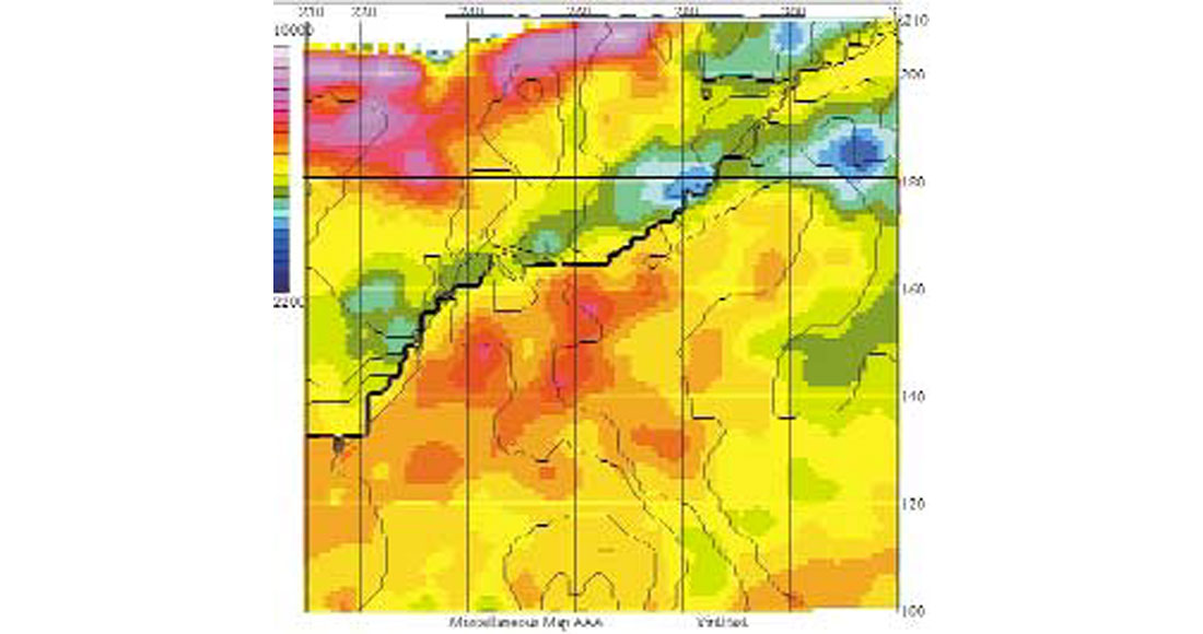
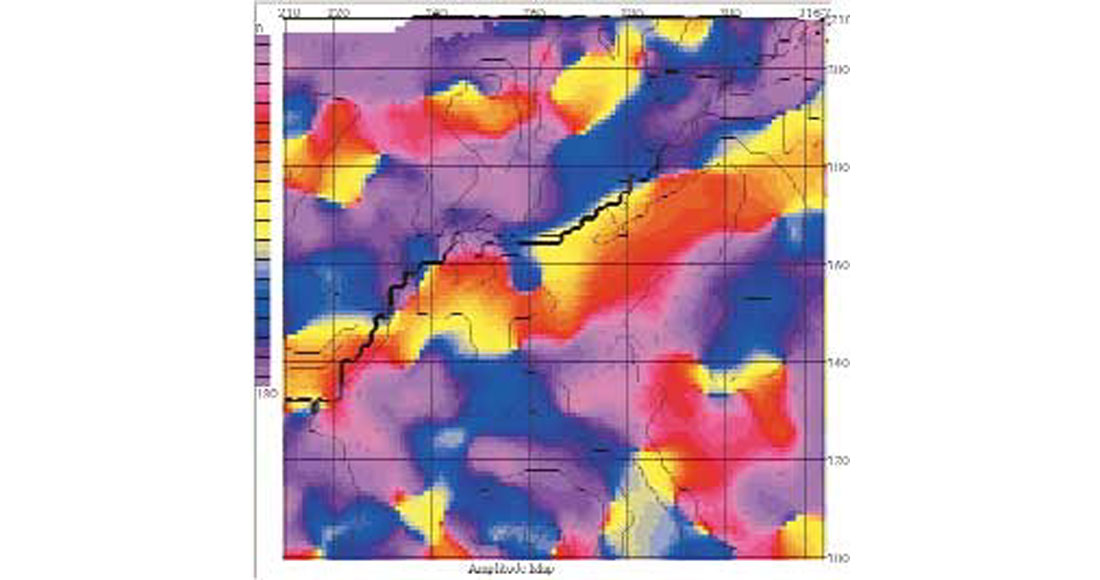
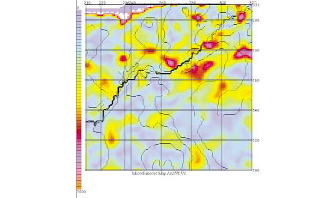
The 3D co-rendering of nine attribute volumes can be illustrated by means of a 2D horizon map, which is of course simply a slice through any given 3D volume filled with nine-dimensional numbers. Figure 1 shows the interval velocity (Vint) for the reservoir unit, a fractured shale about 100 m thick that produces gas, with hydraulic stimulation. Warmer colours are slower Vint; colder colours are faster Vint. Figure 2 shows the azimuth of the fast interval velocity, with yellow being east, red being NE (parallel to the major fault that trends from lower left to upper right), blue being SE; purple pink is north. Figure 3 shows the azimuthal variation in interval velocity, with cold colours being minimal variation and hot colours being maximum variation. The time contours to the top of the reservoir are superimposed.

Method

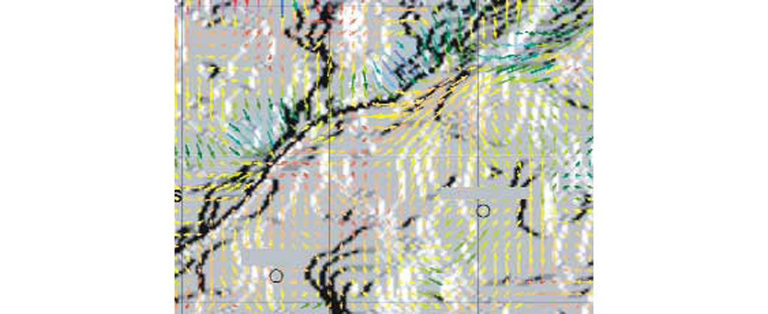
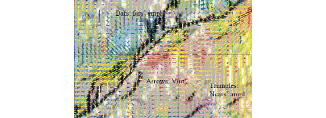
The above three maps are co-rendered here in Figure 4. The coloured arrows represent three numbers: the colour is the magnitude of the interval velocity; the arrow direction is the fast interval velocity direction, and the length of the arrow is the magnitude of the azimuthal variation in interval velocity. By using two more icons, each holding three numbers (magnitude, direction and azimuthal variation), we can co-render nine attributes. Surfer is the off-the-shelf software package from Golden Software that co-rendered the three velocity quantities into one icon, plus one map that is the structure map (rendered by grey shading or contours). The sun angle is the SE corner, 45 degrees off the horizontal plane. Thus the map at the left holds only 4 numbers for each designated “bin”.

Amplitude

PP reflection amplitude is, in general, a six-dimensional quantity. The values of interest are: the zero-offset intercept amplitude; the maximum AVO gradient; the azimuth of the large AVO gradient, the azimuthal variation of the gradient (Max Gradient minus (Minimum gradient), the error (deviation between the ellipse fit and the field data), and the third AVO term (if long offsets are acquired). The azimuthal variation of the third term (the nonlinear portion of the AVO curve) is not well understood, in part because so few field datasets have acquired the proper coverage to systematically analyze it.

Despite amplitude being a six-dimensional number, we are currently using an icon that holds only three numbers, due to our software limitation. It is easy to understand how to construct an icon that holds the six desired numbers, and this represents one avenue of our efforts, to start using icons that hold six dimensional numbers, since velocity is also a 6-D number.

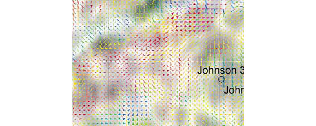
Figure 5 illustrates the co-rendering of nine attributes using three icons. The coloured arrow represents Vint, the coloured triangle represents 5-30 degree angles of incidence AVO gradient, and the coloured bar represents 5-45 degrees angle of incidence. The amplitude icon uses colour to hold the AVO gradient (warm is large, cold colour is small), length to hold the azimuthal variation in AVO (long is large variation, short is small variation), and azimuth to indicate the large AVO gradient azimuth. By inspection of the map, we see where we get the same answer for both ranges of incident angles; and areas where we get different answers for 0- 30 versus 0-45 degrees angle of incidence. Also, we see areas wherein the fast direction is also the bright direction (a large gradient): for example, the red icons in the oval labeled A. Other areas show the fast direction perpendicular to the bright (large gradient) direction: for example, in the oval labeled B. Modeling indicates that the former (the bright direction is the fast direction) is likely to be a higher crack density in the reservoir, while the latter (the bright direction is perpendicular to the fast direction) is more likely to be a higher crack density beneath the reservoir. As is well known, the azimuthal variation in the AVO gradient is influenced by the contrast in the shear-wave splitting (shear-wave birefringence) between the two media at the boundary (and the contrast in delta). While it may be tempting to ascribe the azimuthal variation in the AVO gradient of the base of reservoir reflection to a high crack density in the reservoir itself, it is necessary to remember to look for alternative (outside) indicators of relative crack density in the upper medium and the lower medium. We suggest either multi-component data would serve such a purpose (some split S-wave measurements in and of themselves). But in the lack of such, then PP Vint characterizations (as displayed by 3- or 6- dimensional numbers) are absolutely necessary. The contrast in delta is challenging to determine, but if it does not vary spatially through out the survey, then its effect is simply a constant.

One of the most useful and preferred icon maps is the one termed the “canonical” icon map, since it holds the Velocity, Reflector Amplitude, Velocity, for the Upper medium, the reflector, and the Lower medium. Figure 6 displays the canonical icon map with Vint of the upper medium (the shale reservoir) as the arrow icon, the AVO of the base of reservoir as the triangle (the boundary), and the Vint of the lower medium (the carbonate) as the bar icon. The size of the triangle icon (the amplitude) used the stacked amplitude, although zero-offset intercept would have been preferable. The darker the shade of gray background, the larger the azimuthal variation in the AVO. Our next generation of icons should be capable of holding the five necessary numbers, so that the background can hold the structural contours. The oval indicates a region where the velocities show fast NE and the amplitude is bright NE: the interpretation is that the upper (reservoir) medium is more likely to have the higher crack density. The box indicates a region where the velocities show fast N/S and the amplitude is bright E/W: the interpretation is that the lower medium (the carbonate) is likely to have the greater fracture density. Thus from the map, the relative apparent azimuthal anisotropy of the upper medium and the lower medium is deduced from the two velocity icons (arrow and bar), and compared to the amplitude icon (triangle). Warmer colours are more likely to be associated with hydrocarbons, colder colours are less likely to be associated with hydrocarbons.

All seismic from areas of thick-layers is built of interval, reflector, interval, reflector, etc. To understand the reflector amplitude (AVOA), knowledge of the interval above and the interval below is surely advisable. This is true for PP and for PS and for joint PP&PS.

A further modeling challenge is to handle a change in the apparent fracture azimuth at a boundary of interest – that is, a change in the azimuth of the fast interval velocity direction, at a boundary. At this point, the relative magnitude of the azimuthal anisotropy as well as the relative orientations therein must be taken into account, with the expectation that the largest of the magnitudes will tend to dominate the answer. However, modeling is of course the preferred way to proceed with interpretation.

All the icon maps shown thus far are just 2D slices through a 3D volume filled with icons. Although three icons are used here, the only limit to the number of icons is what the interpreter can handle. What the icon holds is up to the interpreter: multi-component interpreters will of course load their icons (rendered in PP time or depth) to hold PS ampl., PP ampl., S velocity, P velocity, and VP/VS ratio –like numbers, each of which could vary with offset and azimuth. The ability to co-render and interpret all at once nine, eighteen, or thirty-six volumes is proposed as our industry’s next step up. Being able to see our data is the requirement to being able to interpret our data. Obviously, data mining and neural network techniques should be employed to tell the computer which parts of our data we display co-rendered. If all the data is displayed co-rendered, the opacity problem prevents us from seeing anything.

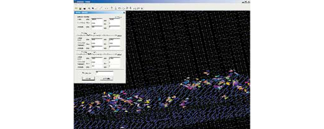
Figure 7 is a screen capture from VIS9D, the prototype 3D volume visualization software package, wherein rectangles, cones, and rhomboids fill a 3-D volume shown on the computer screen, with tilt, swivel, and zoom capabilities. The opacity problem is handled by the user selecting the values of the icons that are desired to be seen.

Obviously, interpreters would prefer rock icons, rather than confetti-like arrows, bars, and triangles. Rock icons, covered in a pending Lynn Inc patent, display sandstones, shales, limestones, and dolomites in their well known geologic symbols, with indicated porosity, pore fill, fracture density, and fracture azimuth as glyphs on the icon. Well control plus seismic can help guide the initial construction of the icon, and rock physics will guide how the high-dimensionality seismic data are transformed into rock icons. The 3D volume will display in an intuitively simple fashion the desired quantities of Structure, Lithology, Porosity, Pore fill (water, gas, or oil, or mixture thereof), uncertainty, fracture azimuth, fracture density, and fracture fill using icons.

Conclusion

Nine-dimensional numbers can be portrayed in map and 3D form, with structure, for interpretation of co-rendered attribute volumes. Efficiency and completeness are better attained when all the relevant and important data can be viewed at the same time.

Acknowledgements

Devon Energy is gratefully acknowledged for permission to show their field data. Vest3D is the pc-based 3D seismic interpretation software Lynn Inc uses. Surfer from Golden Software, Golden, Colorado, is the off-the-shelf software package which enables a user to co-render nine maps (ten maps with structure) into an icon map, with each icon holding three numbers — although woefully inadequate, everyone has to start somewhere. VIS9D is the software prototype package written by Ping Chen that runs on a laptop.