The feasibility of time-lapse gravity and gravity gradient monitoring for Steam Assisted Gravity Drainage (SAGD) Reservoirs is investigated. Two major obstacles have prevented the use of time-lapse gravimetry on small scale reservoirs, namely i) the need for sub-μGal sensitivity, and ii) the high noise levels in the vicinity of the reservoir. In this study, those limitations can both be overcome by using i) a portable superconducting gravimeter, and ii) a pair of instruments under various baseline geometries. This will allow for the measurement of several gravity gradient components, resulting in improved resolution for locating density anomalies, as well as the cancellation of common noise in both instruments. An operational SAGD reservoir in the McMurray Formation is used to forward model the gravity and gravity gradient signatures after 1.25 and 5 years of production, using density changes obtained from seismic monitoring. Signals originating from steam injection and subsequent bitumen migration achieve 2-50 μGal for gravity and 10-400 μGal/km for gravity gradient. The published sensitivity of the iGrav superconducting gravimeter is 0.05 μGal. Even if a more conservative estimate for the sensitivity (e.g., 0.5 μGal) is assumed, time-lapse gravimetry monitoring of SADG reservoirs is achievable. Individual steam chambers can be isolated in the in-line direction of a well pair, but not in the cross-line direction. Reservoir depletion variability across the reservoir can be identified in the gravity gradient signals.
Introduction
Optimized hydrocarbon reservoir management and operations are critical for Canada’s energy market and its global competitiveness. Many procedures such as Steam Assisted Gravity Drainage (SAGD) and hydraulic fracturing have been developed to extract natural resources more efficiently (Economides & Martin, 2008). However, the reservoir processes are often not monitored adequately to observe where fluid migrates and if fluid stays within the reservoir or moves out-ofzone. Deep heavy oil/bitumen reservoirs are produced using SAGD techniques, where steam is injected into the reservoir in the upper well, and displaces bitumen to an underlying, parallel well. The bitumen flow must be monitored spatially and temporally to assess recoverability in the reservoir, and to increase production efficiency. The SAGD process requires considerable energy and water resources, which could be reduced by identifying where low permeability mud layers hinder steam propagation, and avoiding development in those areas (Reitz et al., 2015). In addition, identifying out-of-zone migration earlier could lessen contamination hazards into nearby aquifers.
Current monitoring techniques for bitumen migration include 4D seismic surveys, microseismic surveys, borehole resistivity, temperature and pressure monitoring. 4D seismic surveys provide a comprehensive visualization of the fluid migration, but are costly, and are only conducted every one to three years. Seismic surveys also have limited sensitivity to changes in fluid content, saturation and porosity (Devriese & Oldenburg, 2014). Microseismic monitoring records fracture events, not the fluid migration itself, and is thus an indirect monitoring tool. Borehole monitoring of resistivity, temperature and pressure is restricted to the area immediately surrounding the well. Therefore, a gap exists in short-term monitoring techniques.
The proposed technique utilizes relative gravimetry to monitor spatio-temporal steam and bitumen migration, providing continuous direct monitoring from the surface. The density change from replacing bitumen with steam in the reservoir is monitored by measuring the gravity and gravity gradient signatures. Previously, the feasibility of applying the proposed technique to SAGD reservoirs was hindered by the lack of the required sensitivity in gravimeters, as well as high noise levels. The demand to measure signals at the level of 1 part per billion (or 1 μGal in 981 Gal) and the need to compensate for other processes and noise (Rosat & Hinderer, 2011), (Rosat et al., 2013), which often have higher magnitudes than the targeted signal, create a challenging measurement environment. Both of these limitations can be overcome using superconducting gravimetry in time-lapse gravity gradient surveys, which achieves the sensitivity requirements and greatly reduces noise.
The idea of using time-lapse gravity to monitor density change is not new and several model studies have been conducted as the precision of relative gravimeters increased (Hare et al., 1999; Vasilevskiy and Dashevsky, 2007; Gasperikova and Hoversten, 2008; Krahenbuhl and Li, 2012; Krahenbuhl et al., 2011; Wilson et al., 2012). Time-lapse gravity was first used in field studies in the 2000s (e.g. Ferguson et al., 2007; Davis et al., 2008; Eiken et al., 2008; Jacob et al., 2010), and is inherently a relatively new technology. Recent progress in superconducting gravimeters resulted in a field portable gravimeter, the iGrav by GWR (available since 2010), and is described in Warburton et al. (2010) and Hinderer and Crossley (2004). The iGrav has a reported susceptibility of 1 nanoGal in the frequency domain and 0.05 μGal in the time domain for 1 minute averaging, drifts less than 0.5 μGal/month, and has a noise level of 0.3 μGal/(Hz)½ (GWR Instruments, 2015). In a real environment, a conservative estimate for the value of the susceptibility is 0.5 μGal, which is the value that will be used for the feasibility assessment.
Multiple studies have shown the potential of using time-lapse gravimetry for monitoring purposes, such as SAGD production (Reitz et al., 2015), waterflood production (Brady et al., 2010; Ferguson et al., 2008), gas production (Eiken et al., 2008), CO2 injection (Alnes et al., 2011; Alnes et al., 2008; Dodds et al., 2013), and groundwater extraction (Cogbill et al., 2006; Davis et al., 2008).
This study will demonstrate the feasibility of using time-lapse superconducting gravimetry to continuously and directly monitor bitumen migration in an operational SAGD reservoir. A real SAGD reservoir is forward modeled in the McMurray formation for its gravity and gravity gradient signatures. This study has two objectives:
- What are the gravity and gravity gradient signatures at surface for a real SAGD reservoir, and would a superconducting gravimeter be sensitive to those?
- To what degree can individual steam chambers be isolated through time-lapse gravimetry?
Methodology
Forward Models
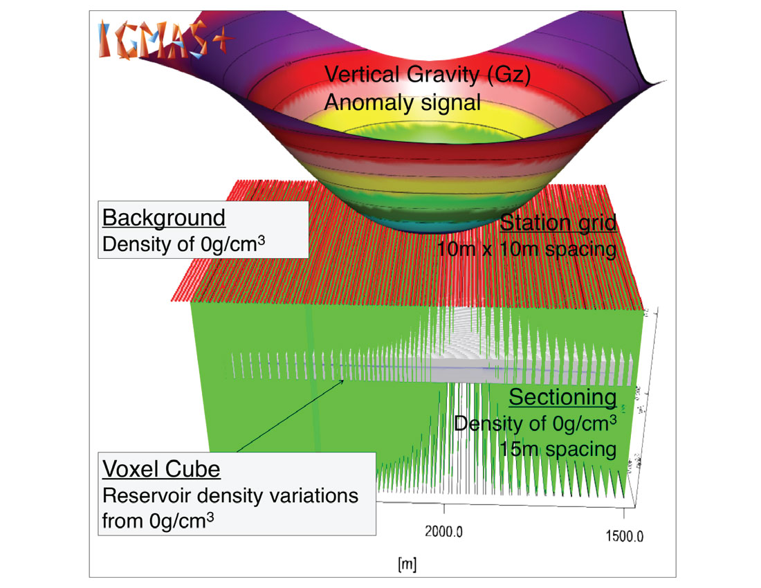
Previous theoretical models have shown that gravimetry is sensitive to the density changes from replacing bitumen with steam (Reitz et al., 2015). Real reservoir density changes will be forward modeled at three time steps (time zero before production, after 1.25 years of production, and after 5 years of production), to analyze the gravity signal components at surface. The provided density data are first organized into voxel cube models. Voxel cube models are created from 2 m3 polyhedrons, each with a given density value and position in space. For each polyhedron, a point mass is calculated with the potential field modelling suite IGMAS (Schmidt et al., 2010). The point mass technique is effective because the vector distance from the point masses to the surface grid stations (>100 m) is significantly greater than the scale of the polyhedrons (2 m3). The voxel cube is sectioned every 15m, and a station grid is overlain on the model with 10m by 10m spacing (Figure 1). As the main concern is relative density changes, the background and section densities are set to 0 g/cm3, with a density variability of -0.30 to 0 g/cm3 for the voxel cube. The triple integral of the point mass in x, y and z is then computed to produce a forward model of the gravity and gravity gradient anomalies for the reservoir at each station grid point.
Gravity and Gravity Gradient
The superconducting gravimeter’s measureable components are vertical gravity (Gz), vertical gravity gradient (Gzz), horizontal cross-line gravity gradient (Gzx), horizontal in-line gravity gradient (Gzy), and the horizontal gradient trend (HGz), which is the combination of the Gzx and Gzy gravity gradients ![]() . Gz and Gzz are predominantly sensitive to vertical changes in density, and Gzx and Gzy are sensitive to lateral density changes. Gravity decays proportionally to the inverse of distance squared, while gravity gradient decays proportionally to the inverse of distance cubed; therefore, gravity gradients are expected to have better spatial resolution and focusing power. However, measuring the gravity gradients requires either the use of two instruments, or varying positions of the gravimeter over time scales that are shorter than steam/bitumen migration processes. A varying baseline gravity gradient survey as performed by Kennedy et al. (2014) for a water reservoir is able to measure the gradients mentioned above.
. Gz and Gzz are predominantly sensitive to vertical changes in density, and Gzx and Gzy are sensitive to lateral density changes. Gravity decays proportionally to the inverse of distance squared, while gravity gradient decays proportionally to the inverse of distance cubed; therefore, gravity gradients are expected to have better spatial resolution and focusing power. However, measuring the gravity gradients requires either the use of two instruments, or varying positions of the gravimeter over time scales that are shorter than steam/bitumen migration processes. A varying baseline gravity gradient survey as performed by Kennedy et al. (2014) for a water reservoir is able to measure the gradients mentioned above.
Reservoir Parameters
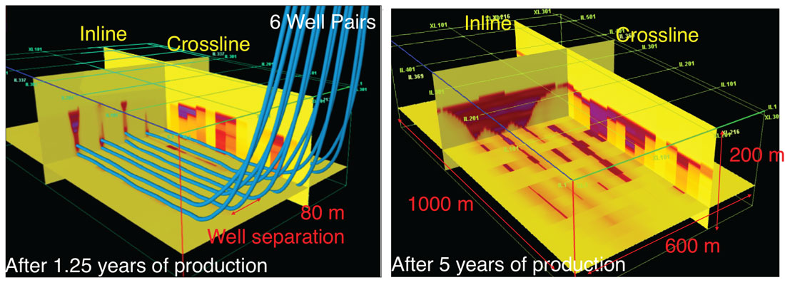
Density data, derived from 3D seismic data of an ongoing SAGD project producing out of the McMurray Formation, is used for the forward models. The density data represents three time steps: the absolute density distribution before production (time zero), after 1.25 years and 5 years of production. The average absolute density of the targeted formation is 2.16 g/cm3, and the density ranges between 1.00 and 3.67 g/cm3. The area under production is 600 m by 1000 m, the targeted depth is 200 m total vertical depth (TVD), and there are six pairs of wells in this area of the reservoir. The sub-horizontal wells are at a TVD of 220 m and have a well separation of 80 m.
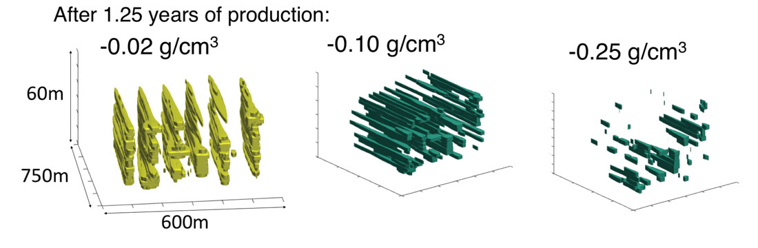
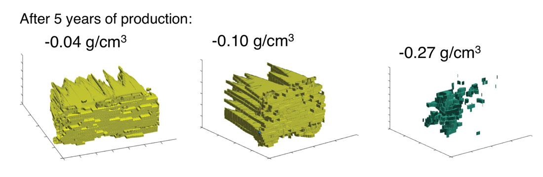
Isosurfaces of the varying density changes were plotted to visualize depletion trends, and identify any sedimentological constraints. For the density changes after 1.25 years of production, the isosurfaces indicate that the density changes extend vertically above and along (in-line direction) the six well paths, but there is no depletion between the well pairs (cross-line direction) (Figure 2). The highest density change is concentrated at the heel of the well, and lessens down the well path to the toe of the well. After five years of production, the isosurfaces show that the density changes extend between the well paths, and that the highest density changes are concentrated at the top of the reservoir, specifically at the heel of the leftmost well pair of the reservoir (Figure 3). Figure 4 illustrates the six well pairs and the density changes in the reservoir, after 1.25 years of production and after 5 years of production.
Results
Real SAGD reservoir parameters are used to create the density models and derive gravity and gravity gradient signals. Five different models are investigated, i) the absolute density distribution at time zero, ii) a single well pair after 1.25 and 5 years of production, and iii) six well pairs after 1.25 and 5 years of production.
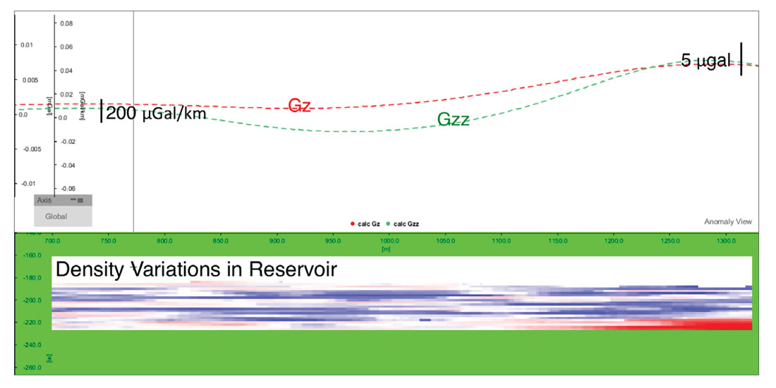
At time zero, a cross section of the reservoir shows density variations throughout, with a positive anomaly on the east side of the reservoir (Figure 5). This absolute density distribution is between 1.00 g/cm3 and 3.67 g/cm3, and reflects the stratigraphy of the formation. Despite this large range, when the densities for different time steps are compared, the static density cancels out, isolating the density changes from the steam migration and bitumen depletion. Figure 5 shows that Gzz is more sensitive than Gz to the baseline density variations in the reservoir. The Gzz signal is approximately 600 μGal/km, and the Gz signal is 3 μGal. These values represent the natural variability of the gravity and gravity gradient signals before production.
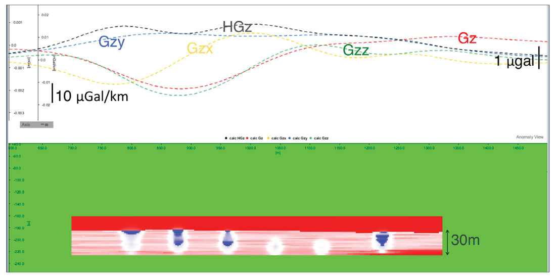
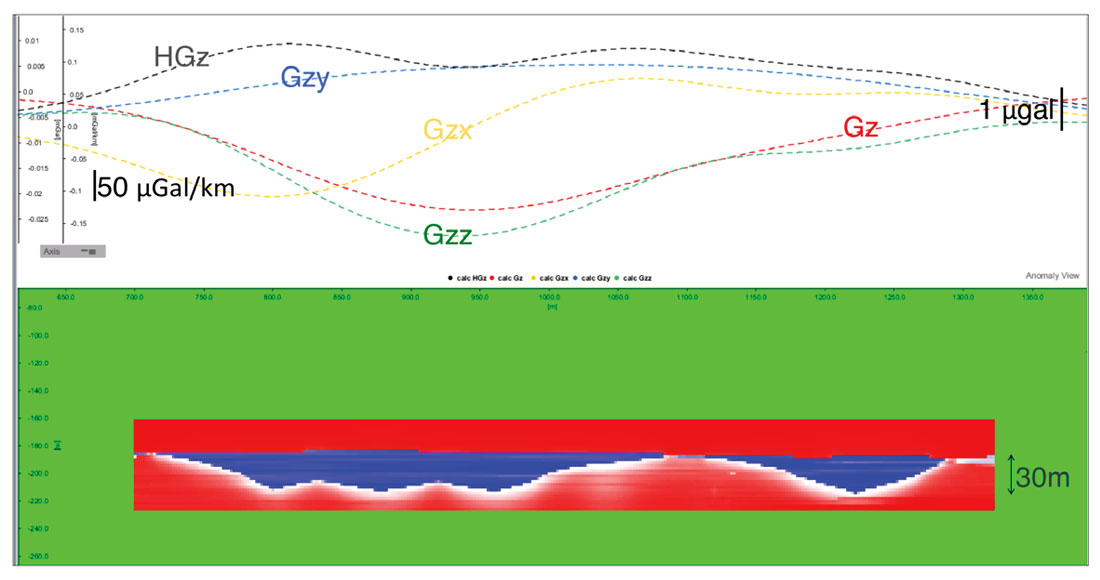
After 1.25 years of production, the cross section of the density changes in the reservoir illustrates the varying degrees of depletion for the six well pairs (Figure 6). The steam chambers for each well grow and affect the reservoir density differently. Gz, Gzz, Gzx, Gzy and HGz are all sensitive to the density changes for the six well pairs, and have stronger responses as the density changes increase. The signals are 1 to 7.5 μGal for gravity, and 2 to 60 μGal/km for gravity gradient. After 5 years of production, the cross section shows that as depletion increases and spreads between the wells, the signals become broader and stronger (Figure 7). Gzz and Gzx are sensitive to the significant depletion on the left side of the reservoir, the lack of depletion in the middle of the reservoir, and the depletion on the right side of the reservoir. The signals are 2 to 50 μGal for gravity, and 10 to 400 μGal/km for gravity gradient.
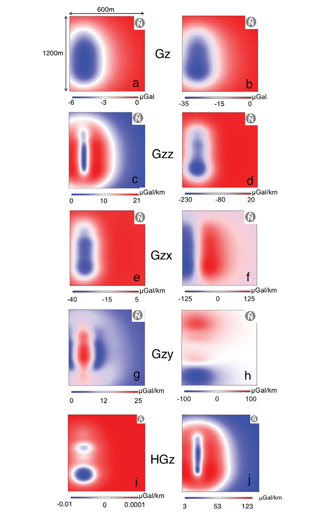
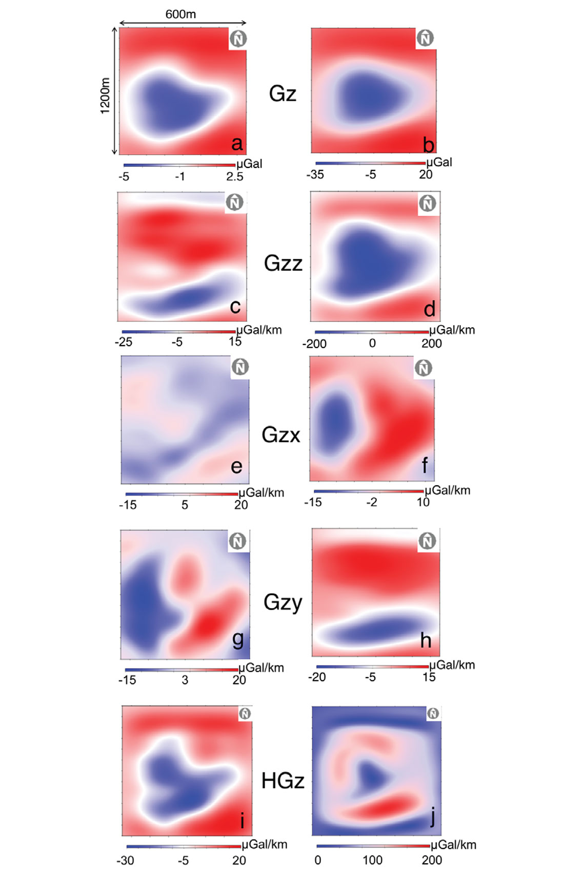
One well pair is selected to show the signal responses in plan view for a single well pair after 1.25 and 5 years of production (Figure 8). All components are sensitive to the density changes, and indicate a directional dependency on reservoir depletion along the well path. Gz (Figure 8a) shows a very broad image of decreasing depletion towards the toe of the well, on the north side, and Gzz (Figure 8c) has a similar but narrower focus on the well path. Gzx (Figure 8e), Gzy (Figure 8g), HGz (Figure 8i) are all sensitive to the variability along the well path, and show the decrease in depletion down the well path. After 5 years of production, all of the signals show a more uniform depletion across the well path, and Gzz (Figure 8d), Gzy (Figure 8h) and HGz (Figure 8j) distinctively resolve the decreasing density changes from the heel to the toe. The gravity gradient signals are sensitive to depletion variations along the well, and are spatially more focused than the gravity signal.
In order to investigate if individual well pairs can be identified when all six well pairs are included, the next model includes all density changes across the six well pairs. The signal responses in plan view for six well pairs generally show the broad depletion trends in the reservoir (Figure 9). Neither after 1.25 years of production nor after 5 years of production, can the gravity and gravity gradient responses differentiate density changes for individual wells. After 1.25 years of production, Gzz (Figure 9c) and HGz (Figure 9i) illustrate the higher depletion in the south part of the reservoir, and varying degrees of density changes in the middle of the reservoir. After 5 years of production, Gz (Figure 9b), Gzz (Figure 9d), Gzy (Figure 9h), and HGz (Figure 9j) each indicate that the reservoir is evenly depleted, with some variability in the south east corner. Gzx (Figure 9f) does not differentiate density changes with respect to individual wells, as the density changes are spread out at the top of the reservoir. HGz is the most illustrative of the density change variability along the well path, and the increase in depletion from 1.25 (Figure 9i) to 5 years of production (Figure 9j).
The density changes isosurfaces indicate that after 1.25 years of production (Figure 2), the highest density changes occur near the heel of the wells, and after 5 years of production (Figure 3), are concentrated in the front left of the reservoir. These trends are apparent in the plan view plots for the gravity and gravity gradient signals, especially for the Gzz (Figure 9d) and HGz signals (Figure 9j). The strongest gravity gradient anomalies are directly linked to the largest density changes in the reservoir.
Discussion
The SAGD process replaces bitumen with steam, driving the bitumen into the underlying production well, and generating -0.30 to 0 g/ cm3 density variations where the reservoir is depleted. After 1.25 years of production, the highest density changes are at the heel of the well, and directly above the injection well path. After five years of production, the density changes extend between the well paths, mostly at the top of the reservoir. These trends occur because the SAGD steam chamber undergoes two growth phases. First the steam chamber rises until it encounters a cap rock barrier, then it spreads laterally and takes an inverted triangle shape. The gravity and gravity gradient signals may be inconclusive during the rising phase as the density changes are limited to the area in the immediate vicinity of the injector (Butler & Stephens, 1981); and impact fluid flow at different stages of production. Small-scale heterogeneities affect steam chamber development near the wellbore at the start of steam injection, and large-scale heterogeneities affect steam chamber development during the entire recovery process (Deschamps et al., 2012). The lack of reservoir depletion in the south-east part of the reservoir indicates that there are large scale heterogeneities that are preventing efficient steam chamber development or bitumen mobilization. Steam injection could have been stopped there to reduce energy use.
The plan view of the gravity and gravity gradient signals for a single well pair can be used to identify specific depletion trends along the well path (Figure 8). For six well pairs, the plan view illustrates the overall reservoir depletion, but it is not possible to identify specific variability across the well pairs (Figure 9). The individual depletion trends for each well, when all six well pairs are combined, overlap because the distance between well pairs is only 80 m. According to a recent modelling study (Reitz et al., 2015) using theoretical reservoir models, separate anomalies for each steam chamber from each well path are distinguishable at minimum separations of 125 m, which is beyond the 80 m separation in the reservoir used herein.
The forward models indicate that Gzz, Gzy, and HGz are the most sensitive parameters to the -0.30 to 0 g/cm3 density changes. The Gz, Gzz, Gzy, and HGz signals for the McMurray formation SAGD project range from 2 to 50 μGal for gravity, and 10 to 400 μGal/km for gravity gradient. Those signals are larger than the conservative iGrav superconducting gravimeter sensitivity, of 0.5 μGal. Thus, there is potential to conduct time-lapse gravity surveys to monitor bitumen flow from SAGD operations, using the iGrav superconducting gravimeter. As a complimentary technique to seismic surveys, time-lapse gravimetry will enable regular monitoring of fluid migration in the reservoir, prevent unnecessary energy consumption, aid in preventing out-of-zone migration, and improve bitumen recovery rates.
This study has not incorporated realistic environmental noise conditions which could originate from SAGD operations, hydrological processes, tidal and atmospheric loading and subsidence. Hence, sensitivity studies in the field must be executed to assess if state-of-the-art relative gravimeters such as the iGrav superconducting gravimeter can achieve the required sub-μGal resolution. The disturbances on site, which include noise from human activity related to production and natural processes, must be quantified and filtered out. The variable baseline method, where two gravimeters are used simultaneously to cancel out signals that are common to both instruments, provides an avenue to cancel out noise (Kennedy et al., 2014).
Conclusions
The depletion trends for a real SAGD reservoir were analyzed by forward modeling the gravity and gravity gradient signals for the density changes after 1.25 and 5 years of production. This study indicates that time-lapse gravimetry is feasible to monitor bitumen migration in a real SAGD reservoir. In particular, the gravity gradient components Gzz, Gzx, Gzy, and HGz are sensitive to vertical and lateral density variations caused by steam injection and bitumen extraction. Reservoir density variations of -0.30 to 0 g/cm3 over a time period of 5 years result in 2 to 50 μGal gravity and 10 to 400 μGal/km gravity gradient signals. Considering the iGrav sensitivity of 0.05 μGal, the iGrav superconducting gravimeter has the potential to be used for time-lapse gravimetry surveys. The variability between the heel and the toe can be monitored for an individual well pair; however, in the cross-line direction, it is not possible to isolate individual well pairs. This is a consequence of the well pair separation of 80 m, which is below the minimum separation of 125 m (Reitz et al., 2015). Despite that limitation, conclusions about the depletion variability across the entire reservoir can be made, which could lead to improved production efficiency. In addition, using superconducting gravimeters to monitor density changes in a reservoir is a relatively inexpensive and non-intrusive method. It enables an improved understanding of steam chamber growth and reservoir heterogeneity, as well as assessing out-of-zone migration flow hazards. While this method will not replace 4D seismic surveys, it provides a viable alternative to characterize SAGD reservoirs, or could be used in synergy with other monitoring techniques.


Join the Conversation
Interested in starting, or contributing to a conversation about an article or issue of the RECORDER? Join our CSEG LinkedIn Group.
Share This Article