Global implications of Arctic climate processes and feedbacks – GLIMPSE

The Arctic exhibits substantial natural variability and climate change simulations suggest that it is a region of the world where climate change as a result of increased greenhouse gas concentrations is likely to be largest. The impacts of this warming, including the melting of sea and inland ice and changes to terrestrial and marine ecosystems are likely to be significant (IPCC, 2001). Projections of future climate changes are complicated by complex interactions and nonlinear feedbacks of the Arctic climate system with other parts of the world as a result of global teleconnections. For this reason, current estimates of future climate changes for the Arctic based on coupled atmosphere-ocean general circulation models (GCMs) vary significantly, indicating a 2 to 6 K warming of the Arctic by the year 2070, with considerable uncertainty and large model-to-model differences (Källén et al., 2001). Not only do the model results disagree in the magnitude of changes, but especially in the regional distribution of these changes.

Understanding how the Earth’s climate system “works”, documenting its variability and determining the extent to which climate is predictable are scientific challenges that have enormous socioeconomic relevance. Because climate is an integrated system of interacting components, climate research requires a perspective view. We therefore seek to find answers to the following questions: What are the global consequences of natural changes in the Arctic climate system? Is the Arctic climate system as sensitive to anthropogenic and external variations as global climate models suggest so far? These questions are investigated at the scale of both the regional (pan-Arctic) and the global scale by improved regional and global climate model simulations. Aside from the fact that the Arctic is a significant component of the global climate system, there is growing evidence that it has a strong influence on and interaction with European climate. For instance, the export of low salinity waters has the potential to influence the overturning cell of the global ocean through control of convection in the subpolar gyres, which in turn feed the North Atlantic and European climate.

Consequently, the main objective of the EU funded project GLIMPSE (Global implications of Arctic climate processes and feedbacks) is to advance our understanding of the key physical processes in the oceans, cryosphere, atmosphere and land and their interactions, including natural variability and abrupt changes, which control Arctic climate and have the potential of global implications and consequences. The goals of the project are to evaluate and improve global and regional climate models and ultimately construct fully coupled regional atmosphere-ocean-ice models. The general aim of GLIMPSE is to improve Europe’s ability to assess climate variability and to develop capabilities for prediction on decadal time scales and on this basis to assist policy makers in their socio-economic decisions on environmental issues. The assessment of potential impacts of climate change has generally so far relied on model data from coarse resolution GCMs which are incapable of resolving spatial scales less than about 300 km. These models include therefore only a limited physical representation of the coupled atmosphere-ice-ocean-land-biosphere system and are generally insufficient in simulating the spatial structure of temperature and precipitation in areas of complex topography (e.g. Greenland and Alaska). The description of regional and local atmospheric circulation systems (narrow jet cores, mesoscale convective systems, see-breeze circulations, shallow stable planetary boundary layers) and the representation of high-frequency processes (e.g. precipitation frequency, intensity distribution, surface wind variability, snow redistribution) are likewise insufficient to provide accurate information. Regional models, on the other hand, depend on accurate boundary conditions that they obtain from the respective driving GCMs. It is therefore essential to improve both global and regional models in parallel. The combined use of coupled GCMs and regional climate models is a powerful resource for improving our understanding of nonlinear decadal scale variations with their large amplitudes, strong regional ocean, sea ice and land surface feedbacks and potential global implications and consequences. This will provide the scientific basis for applying regional climate models to integrated impact studies of climate change scenarios in the Arctic and European North with highly increased credibility on the regional scale.

In general terms, major limitations of studies of climate variability and change in the Arctic have so far been the lack of

1. adequate horizontal and vertical resolution,
2. long-term integrations and
3. coordination between the climate modelling communities involved (European, U.S. and Canadian).

All three issues are addressed in the GLIMPSE project. The coordination goes beyond a strict European effort in that GLIMPSE liaises with U.S. and Canadian groups by coordinating numerical experimentation and data analysis through the definition of common frames of reference for model intercomparison and validation. An ensemble approach is used to provide useful measures of uncertainties by utilising two state-of-the-art coupled general circulation models and three regional climate models (RCMs). Such a comprehensive research effort has never been carried out before. The coordinated efforts within one European project and with the leading American and Canadian groups (Lynch and Curry, 2000) can be expected to enhance our knowledge of model weaknesses related to Arctic processes in a comprehensive way, and based on this, to enable the quantification of uncertainties associated with rapid past and possible future climate changes.

To achieve this, GLIMPSE is:

• addressing and reducing deficiencies in Arctic modelling by the development of improved physical parameterisations of Arctic climate feedbacks in RCMs;
• applying these improved parameterisations into coarser resolution coupled GCMs to determine and understand their global influences;
• assessing the implications of these results for abrupt climate changes on decadal time scales in the past and in the future.

Approach

GLIMPSE is using the following approach:

1. High- resolution climate simulations for the Arctic are conducted with state-of-the-art RCMs with currently used physical parameterisation schemes and validated against a new set of Arctic ground-based, balloon-borne observations plus additional satellite data which have been collected during the SHEBA year (Surface heat budget of the Arctic Ocean, October 1997 to October 1998) to quantify model biases and their uncertainties. The extensive field observations in the high Arctic (Fig. 1) provide by far the best available satellite products for any period in the Arctic and are the foundation for the improvement of atmospheric model parameterisations.

   

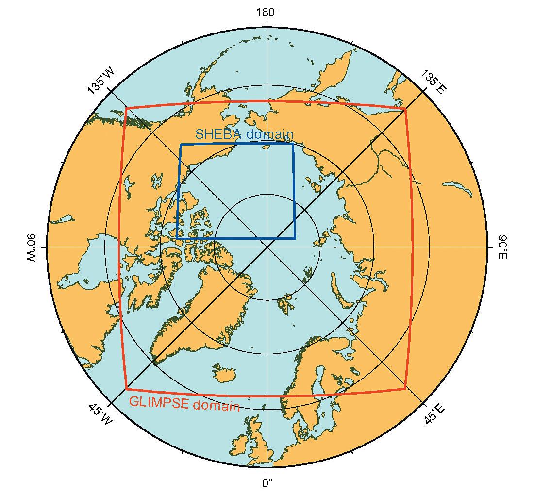
2. Based on comparisons with SHEBA data, parameterisations and the description of feedbacks in RCMs are improved. This includes the description of cloud – water vapour – radiation feedbacks, turbulence schemes in the shallow planetary boundary layer, the hydrological cycle with emphasis on precipitation minus evaporation feedbacks as well as land surface and permafrost processes. Annual runs with the three participating RCMs have been conducted in the pan-Arctic GLIMPSE domain (Fig. 1), and candidates for modifications in the parameterisation have been identified: alternative parameterisations for the albedo over sea ice, snow and snow-covered ice (Költzow et al., 2003; Benkel et al., in prep.), permafrost schemes (investigation of the validity of the zero-flux assumption in the lowest soil layer) and the vertical resolution within the stable boundary layer.
3. The interannual variability and global consequences of the improved description of Arctic climate processes and feedbacks and the regional and temporal patterns connected to decadal to centennial variability in the Arctic are investigated in long (500 years) GCM simulations with fixed and variable external forcing. We have carried out a simulation under the influence of a comprehensive set of natural and anthropogenic forcings: volcanic and anthropogenic aerosol, solar variability, greenhouse gases and land use changes for the period 1500 to 2000. It will be this part of the project that will be described in detail below. The aim is to assess variability in GCMs and RCMs as a function of model formulation, external forcing processes and internal variability, to allow for the determination of uncertainties in climate scenarios, to assess the risk of climate change due to regional feedbacks, and ultimately, to develop fully coupled atmosphere-ice-ocean models with improved parameterisations for the whole Arctic.
4. Regional models are driven with time slices from the coupled GCM simulations described above to assess the potential of rapid regional climate shifts like the “Little Ice Age” on socioeconomic systems in Europe and particularly in the Arctic.

Partners

The GLIMPSE consortium consists of 7 partners: Alfred Wegener Institute for Polar and Marine Re-search, Potsdam (AWI), coordinator: Klaus Dethloff, Norwegian Meteorological Institute, Oslo (DNMI), Rossby Centre, Swedish Meteorological and Hydrological Institute, Norrköping (SMHI), Danish Meteorological Institute, Copenhagen (DMI), Stockholm University, Department of Earth Science and Geography, University of Tromsö, Norwegian College of Fishery Science, Tromsö (NCFS), Institute for Coastal Research, GKSS Research Centre, Geesthacht (GKSS).

A public GLIMPSE web site has been set up at http://www.awi-potsdam.de/atmo/glimpse/.

A 500 year climate simulation incorporating a comprehensive set of forcings

Introduction

Considerable attention has recently been paid to the evolution of climate and in particular temperature over the last couple of centuries. Since we do not have a sufficient amount of direct measurements prior to about 1850, proxy data (tree rings, ice cores, corals and historical documents) must be used to assess the climate of earlier times. In order to put the temperature evolution of the 20th century into a longer-term context, estimates of natural variability (internal variations of the climate system in absence of external forcings) as well as forced variability (both natural and anthropogenic) are required. Several of such multi-century reconstructions exist and have received considerable attention, e.g. Mann et al.’s “hockey stick” (Mann et al., 1999). Others have recently been presented e.g. by Huang et al. (2000), Briffa et al. (2001) and Esper et al. (2002), the first based on borehole temperatures, the other two on tree rings. An extensive review paper by Jones and Mann (2004) puts these and other estimates of past temperature variability in context. Recently, using idealised proxy records obtained from a coupled model simulation, von Storch et al. (2004) argued that centennial variability may have been larger than these empirical reconstructions indicate. Climate reconstructions based on proxies have inherent uncertainties. The resolvable variables and the regions for which these reconstructions are derived are not necessarily identical. As an example, tree growth is sensitive to temperature and precipitation, but the actual ring thicknesses will depend on which quantity is the limiting factor. In such a situation, multi-century transient climate simulations can help us to gain understanding of the temperature variations of past centuries and of the underlying physical processes when conducted with state-of-the-art coupled general circulation models. Results of these simulations agree broadly with the reconstructions of Mann et al. (1999) and other authors in that there was an extended period until the mid-19th century with temperatures lower than present, often (somewhat incorrectly, see Jones and Mann, 2004) termed the Little Ice Age (LIA). In order to conduct such a transient simulation, it is essential to be able to quantify all the various natural and anthropogenic forcings that are at play as realistic as possible.

Our work differs from previous publications by two aspects: we have included a latitude dependence of volcanic aerosol and a description of land use changes in the forcing. Aspects of the forcing data sets are described in detail in Stendel et al. (2004), and we give only a short overview here.

Model

In this study, we use the coupled ocean-atmosphere model ECHAM4-OPYC3. Its atmospheric part, ECHAM4, is described in Roeckner et al. (1999). The ocean model is an extended version of the OPYC model (Oberhuber, 1993), which consists of sub-models for the interior ocean, the surface mixed layer and sea-ice. Ocean and atmosphere are quasi- synchronously coupled, exchanging information once per day. An annual flux correction for freshwater and momentum is applied, based on present-day climate conditions. Further details about the model can be found, e.g., in Stendel et al. (2000), and references therein.

Forcings

Natural forcings include solar irradiation variability and volcanic emissions, and anthropogenic forcings include time-dependent concentrations of greenhouse gases and chlorofluorocarbons (CFCs), land use changes and a simplified tropospheric sulphur cycle. Orbital variations can be neglected due to the comparatively short period that is investigated here.

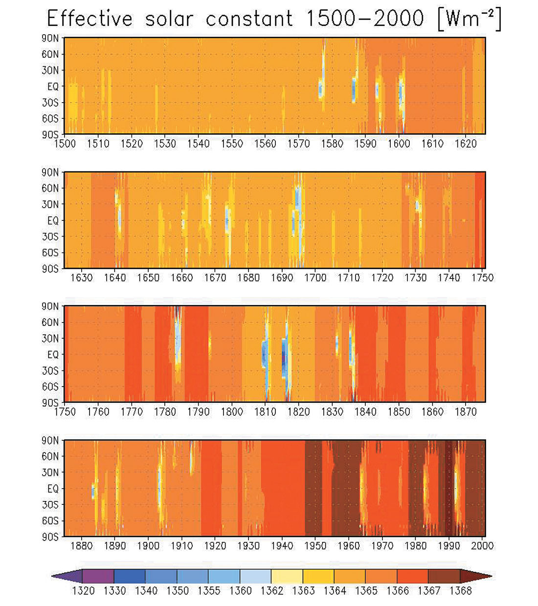
For solar irradiation, we used the data set of Lean et al. (1995, updated), covering the period 1500 to 2000 with annual resolution. Alow-frequency trend with an increase of total solar irradiation by about 0.2% from the Maunder Minimum until today is visible, see Fig. 2). Apart from volcanic activity (see below), the figure clearly shows several minima in solar irradiance, in particular the Spörer Minimum in the first part of the 16th century, the well-known Maunder Minimum (about 1650 to 1715), and the Dalton Minimum in the early 19th century. Since then, a general increase in irradiance is evident.

The Robertson et al., (2001) annually and latitude-resolving volcanic optical depth dataset has been used for the period 1500 to 1889. This index is obtained from the observation of sulfate aerosol in ice cores. From these, one can calculate the perturbation in optical depth following the procedure of Stothers (1984), which can be expressed as anomalous radiative forcings at the tropopause for the solar and long wave part following Andronova et al. (1999). From 1890 on, we have used the monthly-resolved data of Ammann et al. (2003). Note that there is considerable uncertainty about the actual amount of volcanic aerosol ejected into the stratosphere, resulting in a difference by a factor of 6 between two recent datasets (Robertson et al., 2001 and Crowley, 2000) even for well-documented eruptions like Tambora, 1815.

The annual concentrations of greenhouse gases (CO2, CH4 and N2O) are also taken from Robertson et al., (2001). They have been obtained from ice core data. For the well-mixed carbon dioxide, one measurement from Law Dome (Antarctica) is sufficient. For methane, which is less well mixed, time series from both hemispheres have been averaged, and for N2O, an average of a number of Antarctic records was used. The concentrations of halocarbons (CFCs) have been taken from observations described in the 3rd IPCC assessment report (Nakicenovic et al., 2000).

In contrast to previous studies, we also take into account the effects of anthropogenic vegetation changes. We use the so-called HYDE “A” data set (Klein Goldewijk, 2001) which includes on a 0.5° by 0.5° grid croplands as well as areas used as pasture, which are estimated from population densities as well as estimates of livestock, gross domestic product and industrial production. The vegetation classes were assigned to the ECHAM vegetation classes (Claussen, 1994; Hagemann et al. 1999) and interpolated to the model grid. Then, differences to present-day conditions for background albedo, forest and vegetation ratio, leaf area index and surface roughness are determined. The dataset shows large-scale deforestation in Europe in the 18th century, in the western U.S. in the second half of the 19th century and, more recently in East Asia (not shown here).

ECHAM4 has a simplified tropospheric sulfur cycle described in detail in Roeckner et al. (1999). Sulfur emissions with their actual geographical positions are given as decadal means from 1860 on. The transformation to sulfate, semi-Lagrangian transport of the sulfate aerosols as well as dry and wet deposition of sulfate particles from the atmosphere (Feichter et al., 1996) are taken into account. The indirect aerosol effect on cloud albedo, following Boucher and Lohmann (1995) and Lohmann and Feichter (1997), is also included. In addition, the tropospheric ozone concentration is allowed to vary as a result of prescribed concentrations of anthropogenic precursor gases (OH-, NO3-, O3, H2O2) whose concentrations are given for 1860 and 1985 and linearly interpolated in between (Roelofs and Lelieveld, 1995).

Experiment setup

The model was spun down from present-day to AD1500 conditions by applying the pre-industrial values of all the forcings described above. After a period of 500 years, the model variables had asymptotically approached nearly constant values. From this starting point, an unforced control simulation and a forced experiment including all forcings have been run for 500 years each. For an estimation of the effect of land-use changes, an additional simulation was run for the last three hundred years using constant vegetation for 1700.

Evolution of surface temperature and comparison to proxy data

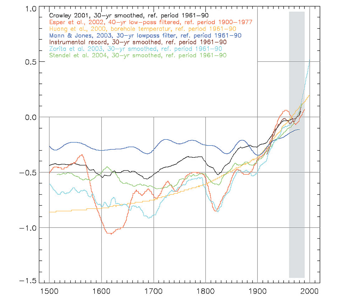
In Fig. 3, we show the simulated evolution of global near- surface temperature with reconstructions from instrumental observations, an energy balance model (Crowley, 2001), dendrochronologies (Esper et al., 2002), borehole data (Huang et al., 2000), Mann et al.’s (2003) multi-proxy reconstruction and a model simulation with the same atmospheric model in coarser resolution, but a different ocean model (Zorita et al., 2004). Temperatures in our study generally follow the proxy data, with negative anomalies during the Late Maunder Minimum (late 17th and early 18th century) and around 1830, as well as a strong temperature increase since the mid-19th century. Compared to the simulation by Zorita et al., the negative anomalies in our simulation are smaller. This can be explained by the considerably larger solar variability and volcanic forcing that has been used in their data set. Large volcanic eruptions can influence global temperature on a time scale of several years. The most striking example follows the eruption of Tambora in 1815. The “year without a summer” 1816 following this event (Harington, 1992; Robock, 1994) is evident in the simulation (not shown). Other examples of major volcanic events leaving an imprint in the global temperature curve include Laki on Iceland in 1783 and Krakatoa (Indonesia) in 1883. Also the “1809 event” (clearly visible in ice cores, the responsible volcano remaining unknown, see Budner and Cole- Dai, 1993) can be identified. While the model is able to depict the direct radiative effects of large volcanic eruptions, it fails to simulate flow anomalies triggered by tropical eruptions (Robock and Mao, 1995; Shindell et al., 2001b) which tend to cool the polar stratosphere and therefore strengthen the polar vortex, leading to warmer than normal temperatures in the winter following such an eruption in large parts of Europe. Warm periods in the early 17th century and in the second half of the 18th century are likely caused by increased solar irradiation.

To assess the regional distribution of anomalies during the Late Maunder Minimum (LMM), we compare simulated and reconstructed (Luterbacher et al., 2003) seasonal temperature anomalies over Europe from the 200 year average 1500-1700. Fig. 4 shows winter (DJF) temperatures as an example. According to the reconstruction, the LMM period was characterised by colder than average winter conditions over most of the continent and positive anomalies over most of Scandinavia. The model is able to depict this general pattern and thus seems to have skill to simulate large scale regional climate changes. Simulated cold anomalies in summer, however, extend too far south (not shown). The general increase of blocking situations during the LMM (compare Luterbacher, 2001) is also simulated.

To assess the effect of vegetation changes, we have conducted a sensitivity experiment where background albedo, forest and vegetation ratio, leaf area index and surface roughness were held constant at 1700 values. While the global effect of vegetation changes is small (less than 0.1 K), differences up to -0.3 K are simulated over Europe in the 18th and over the US Great Plains in the 19th century with the full forcing simulation being colder. There is also a modest reduction in temperature over south eastern Asia in the first half of the 20th century. This is in agreement with estimates from transient experiments by Matthews et al. (2003), but smaller than the results reported by Matthews et al. (2004) using an interactively coupled vegetation model.

Multidecadal circulation anomalies

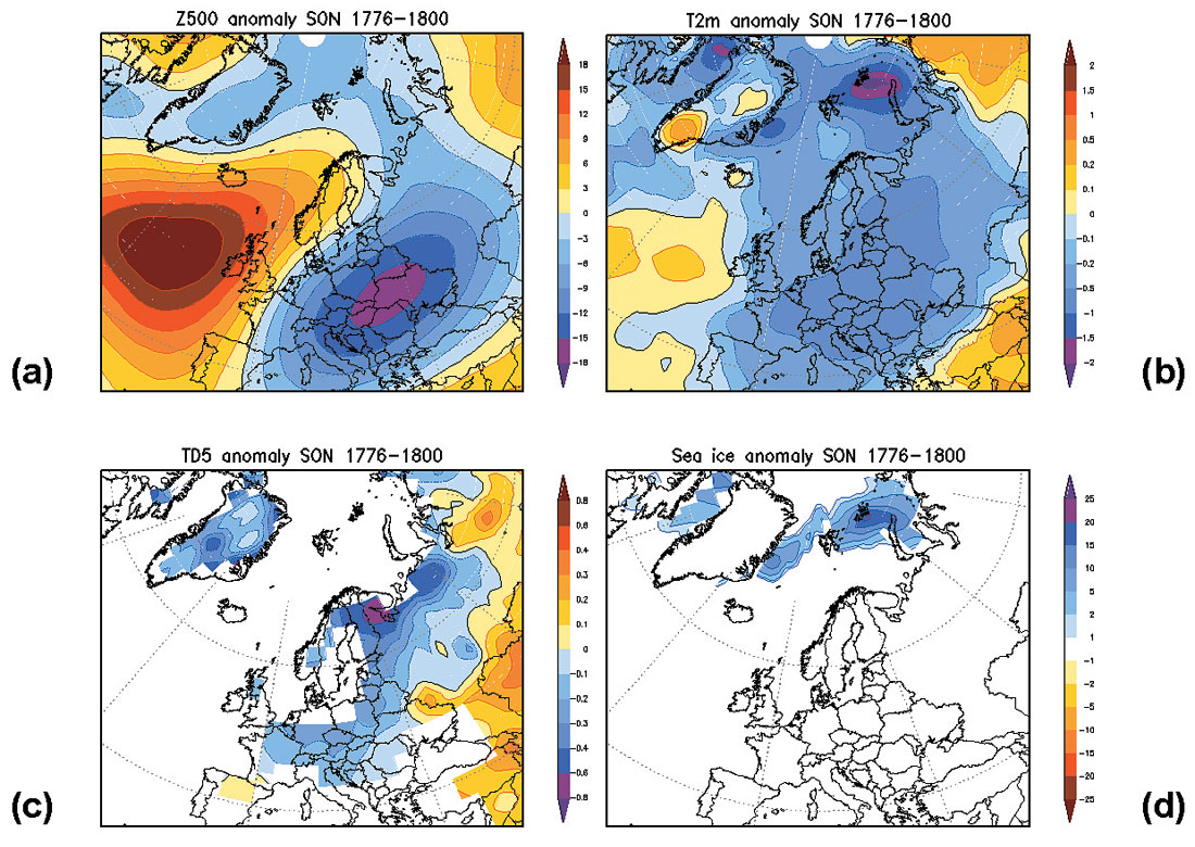
In order to further assess typical Atlantic-European circulation anomalies in the model, a time series of European temperature anomalies was constructed, covering the same area as the Luterbacher et al. data. From this time series, several 25 year segments were chosen: a particularly cold period centred on 1788, a warm spell centred on 1612 and two periods covering the onset (1666-1690) and the end (1691-1715) of the LMM. For these periods, temperature (both near-surface and deep-soil), precipitation, sea ice cover and 500 hPa height (sea level pressure is very similar) were compared to the average 1500-1700. As an example, we here show these fields for autumn of the second cold period (Fig. 5). During cold periods in winter (DJF), positive sea ice anomalies are found in the Greenland / Iceland region. Over Eurasia, we find a general weakening of the zonal circulation by either anomalous high pressure in the polar region or anomalous low pressure over most of Eurasia. Both types of circulation anomalies favour positive sea ice anomalies near Iceland and along Greenland’s east coast. There are also large cold anomalies over Northeast Europe due to anomalous snow cover. In summer (JJA), cold periods are also characterised by a simulated weakening of the zonal circulation, caused by either anomalous high pressure over Greenland or anomalous low pressure over most of Europe/Asia. Both circulation patterns go along with a southwest displacement (and probably weakening) of the Azores high and generally tend to transport cool Atlantic air masses into most of Europe. The most striking circulation anomalies occur in autumn (SON) where, even in the 25 year average, a 500 hPa anomaly of more than 20 gpm is simulated over Western Europe.

The North Atlantic Oscillation (NAO)

There is evidence from reconstructions by Luterbacher et al. (2002) and Glück and Stockton (2001) for a strong increase in zonality since the mid-19th century. Such an increase for the last 150 years - with the notable exception of the 1940s that were characterised by low NAO indices in the European-Atlantic region – is also visible in the first EOF (explaining 37% of the variance) of our simulation (not shown here). Corroborating results by Zorita et al. (2004) - obtained with quite a different forcing - we find a shift of the NAO index from negative to positive values approximately halfway through the LMM. A circulation pattern with high pressure over the British Isles is given by EOF2, which explains almost a fifth of the variance. The corresponding PC has a large loading during most of the LMM, thus corroborating our findings about the increase of blocking patterns discussed above.

The thermohaline circulation

Rahmstorf and Ganopolsky (1999) report of a general slowing down of the Atlantic thermohaline circulation (THC) under global warming conditions, caused by the decrease of surface water density by either increased warming or an anomalous freshwater flux. However, in ECHAM4/OPYC, we do not find a particular sensitivity to changes in the forcing. This is a particular property of this model: Under warming conditions, the stability of the THC is caused by a poleward transport of anomalously saline water (caused by anomalous evaporation) from the tropical Atlantic. This remote effect is able to compensate for the local effects in the North Atlantic which tend to decrease the density of surface water through warming and increase in freshwater flux (Latif et al., 2000). The opposite is true for cooling conditions. Therefore, the THC remains rather stable throughout the simulation.

Discussion

Near-surface temperatures as well as deep soil temperatures well below the long-term average are simulated for extended periods, including the LMM. We find an accompanying decrease in solar irradiation and an increase in volcanic activity during the same periods. The fact that there is a clear response in our simulation despite the relatively small forcing (compared to Zorita et al., 2004) can be explained by the large impact of extratropical volcanoes on high-latitude temperatures (see e.g. Laki on Iceland in 1784) in the solar part of the spectrum. Latitudinal resolution (as well as correct placement in time) of the volcanic aerosol is therefore essential. As suggested by Shindell et al. (2001a), a decrease in radiative forcing, caused by less solar irradiation and/or volcanic aerosol, leads to a decrease in the upper tropospheric temperature gradient between tropics and high latitudes, a decreased northward momentum transport and therefore to a weakening of the NAO. This is the case in ECHAM despite the rather simplified representation of the stratosphere. Such quasipersistent circulation anomalies could lead to positive sea ice anomalies east of Greenland and around Iceland, regions that are particularly sensitive to circulation changes in ECHAM (Stendel et al., 2000), but probably also in reality. There is historical evidence (e.g., Lamb, 1982) for above average ice conditions around Iceland during the LMM. Once such a cold anomaly has evolved, it can persist for quite some time, perhaps influenced from the lower boundary by widespread below average soil temperatures. The effect may be further enhanced by freezing of previously unfrozen ground in the transition zone to permafrost. Such a weakening of the zonal circulation could, on average, persist for several years and lead to cold conditions in Europe except in summer, where the thawing of the upper layer acts as a blocker from the deeper frozen soils. It would also go along with an increase of blocking situations. It remains to be examined if there is a dependence on resolution, since the remarkable increase in blockings is not apparent in the coarser resolution (T30) in Zorita et al.’s simulation.

In contrast to the mechanisms discussed above, the weakening of the ocean gyre circulation, as described in Zorita et al. (2004) does not seem to play a prominent role for the present model, as the local freshening in the northern oceans is compensated by the transport of saline waters from the tropics. The level of externally forced variability in our simulation is larger than in Crowley’s (2000) energy balance model. It is also larger than several reconstructions suggest, in particular that of Mann and Jones (2003). In our reconstruction, the LMM is the coldest period of the past 500 years which is also true for the Zorita et al. simulation with much larger forcing than used here. We conclude that state-of-the art climate models are able to simulate multidecadal circulation anomalies such as the LMM, even under conservative forcing assumptions. In view of past climate evolution, the warm conditions at the end of the 20th century are highly unusual and unprecedented for at least the last five centuries.

In comparison to high resolution empirical climate reconstructions, the model is able to some extent to simulate regional climate anomalies, mainly in winter (DJF), suggesting that there is a memory effect for soil moisture that is not adequately covered in ECHAM’s rather simple soil scheme. However, as can be seen in the years following large volcanic eruptions, it mainly reacts to the reduced insolation, but fails to reproduce the dynamical effects following such forcing anomalies.

Acknowledgements

GLIMPSE is a research project (contract EVK2-CT-2002-00164) supported by the European Commission under the 5th Framework Programme. Results by the following GLIMPSE participants are discussed or quoted: A. Benkel, J.H. Christensen, K. Dethloff, M.Ø. Költzow, P. Kuhry, I.A. Mogensen, B. Rockel and H. von Storch.

Corresponding author: Dr. Martin Stendel (mas@dmi.dk)

This article was first published in ‘EGGS’, newsletter of the European Geosciences Union (http://static.egu.eu/static/5343/newsletter/eggs/eggs_12.pdf), Issue 12, July 2005, and published here with permission from EGU.