Geostatistical Depth Mapping: Integration of Seismic Times with Well Tops

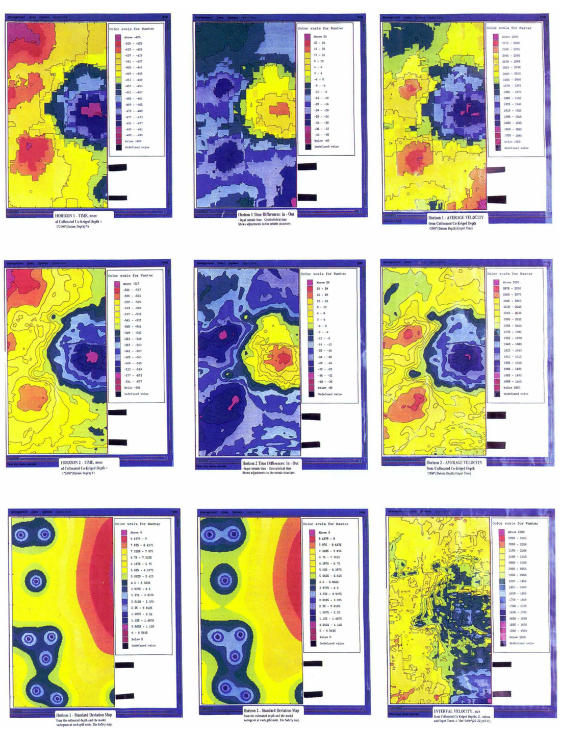
A perpetual exploration problem is to produce depth maps useful for the goals of both geologists and geophysicists and to accurately derive a target depth estimate at a proposed well location. A case history whereby seismic horizon times and well tops are combined to estimate depth using the collocated co-kriging method is graphically illustrated. Directional anisotropy is identified and taken into account. Although geological structural surfaces can be spatially nonstationary, this is usually not a problem over small areas of investigation. Useful physical information can be extracted from the results. Back calculated average velocity using the seismic processing datum, input time horizon and the depth map provides a check on the physical results. Applying the datum and replacement velocity to the depth map yields an adjusted time horizon. Input and adjusted time differences are computed. These derived data are used as a quality control, for isochron mapping, and for flattening seismic data.

This poster paper was shown at the May, 1996 CSEG Convention. The format is necessarily informal.

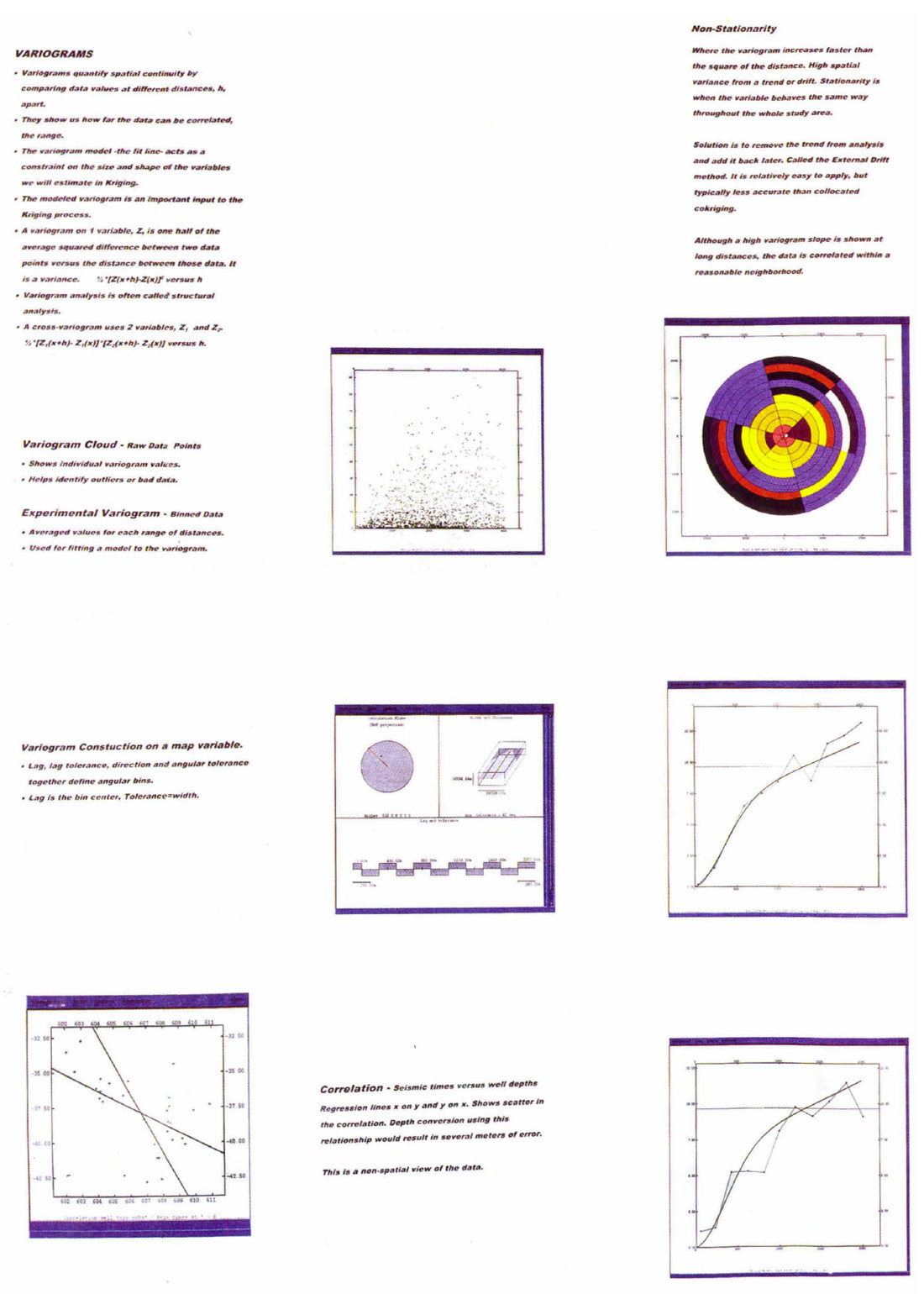
Methodology

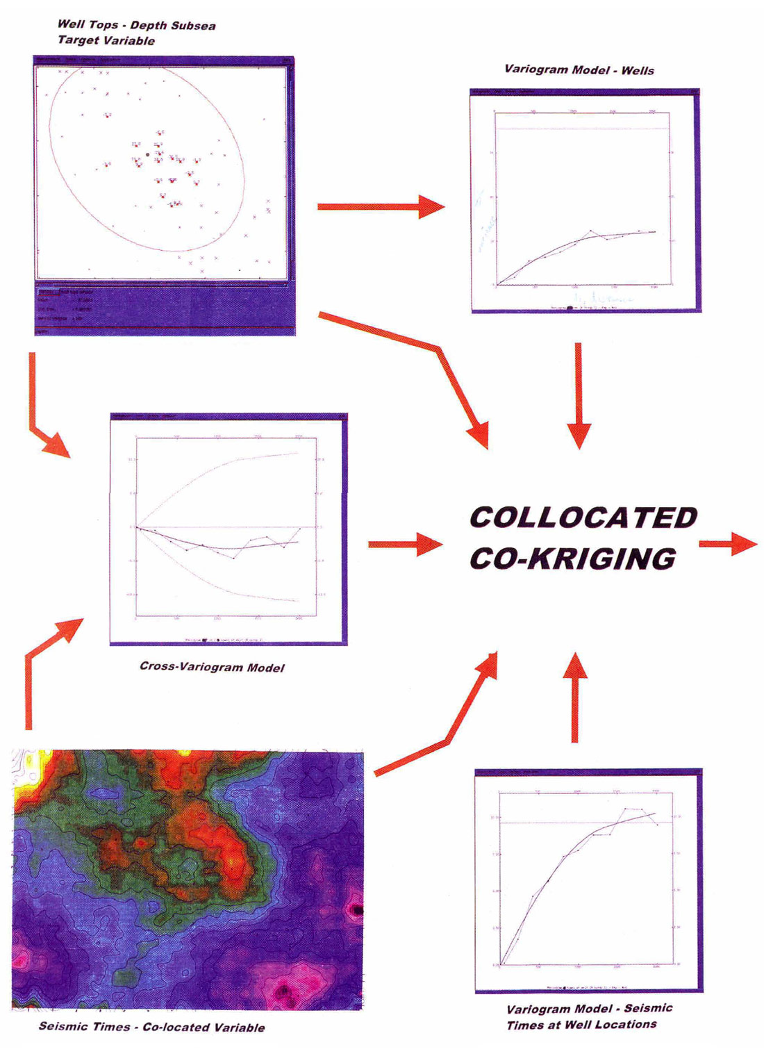
The first 2 panels illustrate the method of Collocated Co-Kriging. The input data are subsea well tops and seismic structure times. These data are continuous random variables and are assumed to be accurate. Both sample the underlying physical phenomenon. The wells are sparse and provide the target variable for co-Kriging. The seismic data is dense, thus providing information to fill the inter-well surface. Do the data adequately sample the structure surface?

Semivariograms are computed for each variable at the well location and a cross-variogram links the 2 variables. As illustrated in the figures, the variogram cloud and the experimental variogram come from the data. A variogram model is fit to the 3 experimental variograms and is used to weight the Kriging interpolation. The model variogram must be valid for all 3 variograms to solve the Kriging matrix. This is the positive definiteness criterion for matrix inversion. Most of the practitioner's effort and experience is required at the variogram fitting stage of the process.

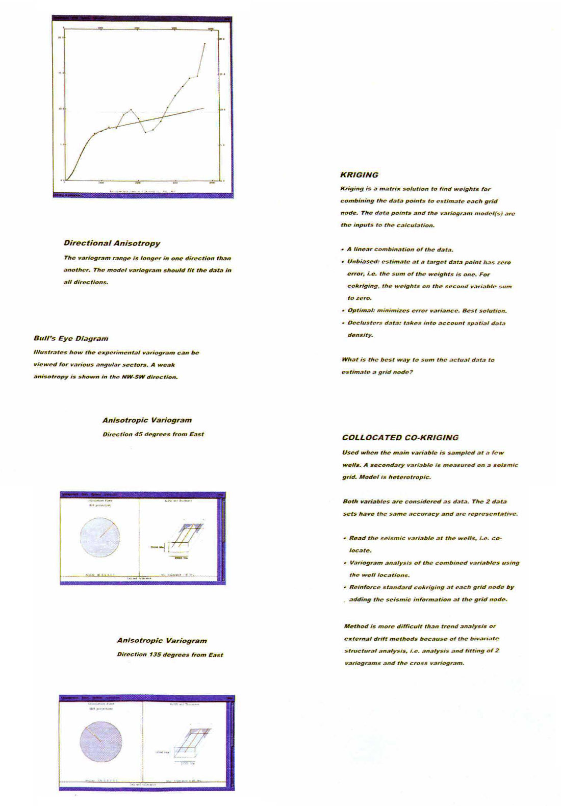
As stated in the figures, the variograms describe the continuity of the phenomenon. The directions of minimum and maximum continuity if present can be described by variograms. This is geometrical anisotropy. Typically a practitioner will attempt to identify and quantify anisotropy. Using the ISATIS software package from Geomath, bullseye plots, variogram maps and a series of narrow angle variograms with several azimuths are generated. Often with sparse well sets, anisotropy is difficult to quantify and model with certainty. Input maps or the interpreter's expectations can help. If present, it is always worth comparing final maps with and without modeled anisotropy to assess the impact. Final results are typically insensitive to small changes in the variogram model. Unless there is a strong evidence of geometric anisotropy, one need not apply it.

Collocated co-Kriging is a powerful estimation technique to linearly combine the variables. The variogram model is fit for the 2 variables collocated at the well locations. The variogram model at the wells best describes the spatial shape. Kriging now has information on how to combine the data as the separation between grid nodes being estimated and the hard data increases. The dense seismic data reinforces the co-Kriging away from well locations. The correlation between time and depth impacts the seismic detail integrated into the depth map. A well top is honored when a grid node is at a well location. One significant property of Kriging is to de-cluster data. A grid node estimated between a cluster of data and an isolated point will not be dominated by the cluster.

Case 1

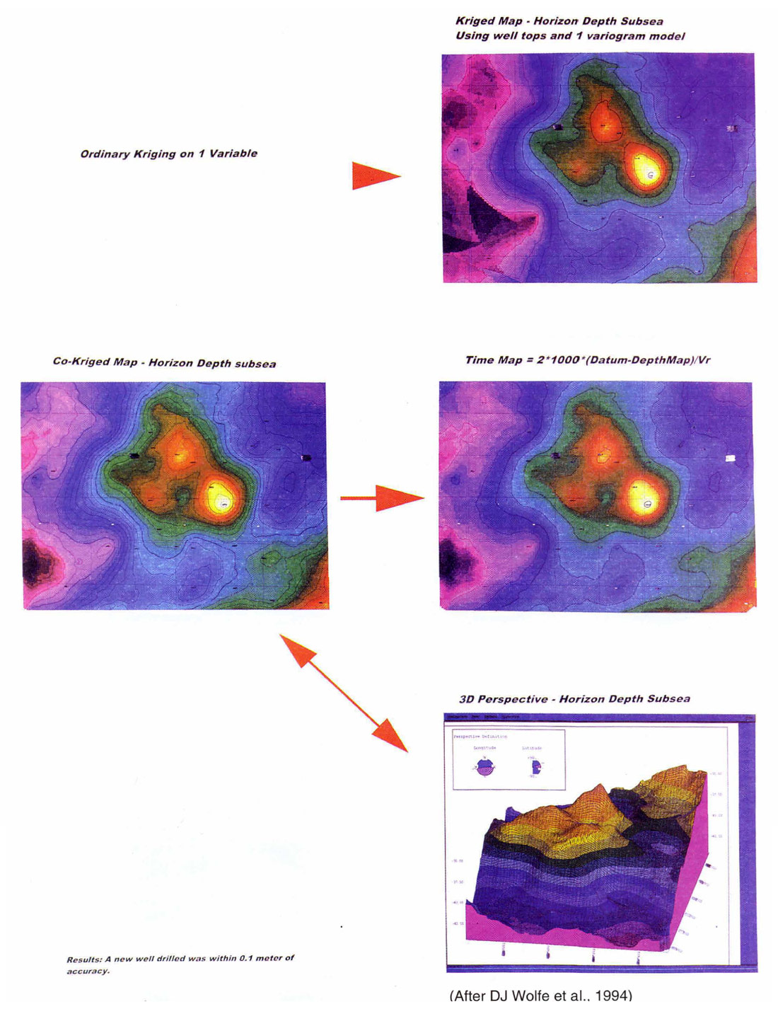
The study shown in the flowchart is an Alberta Cretaceous horizon in an 8 square kilometre area. The result is a subsea depth structure map on the horizon. Comparing a depth map based on Kriged well tops illustrates the added detail from applying collocated co-Kriging. Approximately 55 wells were utilised in the solution. The co-Kriged depth map was used to compute an adjusted time horizon to provide a stratigraphic datum for further seismic interpretation.

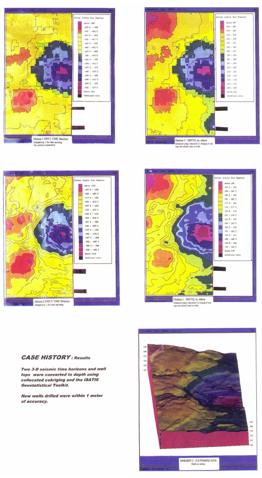
Case 2

The study area is in the Cretaceous Heavy oil area of the Western Canadian Basin. The area is around 10 square kilometres and is a subset of a the full study area. Fourteen wells were used. The input horizon time structures do not tie the depth structure reasonably. After collocated co-Kriging, the subsea depth structures tie the wells. On the deep horizon, the 2 wells in the northwest area of the figures best illustrate the result. Two subsequent wells were drilled on the survey and were within a meter of the predicted depths. The new wells are not shown. For your information, the shallow horizon was not smoothed before the study.

The depth maps can provide us with additional information. The computed average velocity shows the velocity trend where the 2 wells and the time horizon did not tie. Interval velocities were computed between the 2 horizons. The interval velocity decreases down dip. If the valley is filled with lower velocity material than the crest of the structure, is this depositional or diagenetic?

The standard deviation plots are only used as a qualitative measure of uncertainty. The absolute estimation errors are not accurate since they are computed based on the model and the estimate. Relative changes are a guide to safety. Drilling is the only way to measure the depth error.

Comments on Collocated Co-Kriging for Depth Mapping

This method can be highly accurate and useful, but has a tendency to produce a map smoother than reality. The technique tends toward the mean or safest value at each grid node. It minimizes error. It is the most probable answer given the data. With faulting or very rough structures the resultant depth map may be unappealing. Preserving the roughness of the surface and faults is possible through alternate Geostatistical strategies and is a subject for a full paper.

Calculating volumetrics is a logical use of depth maps. Because Kriging tends toward the mean, the gross rock volumes computed will be underestimated. The estimate will be near the 50% probability. A technique called co-simulation is one used to generate the cumulative probability distribution of volume between the surface and a contact.

The number of wells tops available is a data dependent limiting factor on the technique. Contrast 2 examples. Five wells were adequate in one case where the correlation was excellent between time and depth. Another case with 17 wells in an area of moderate structural relief presented a difficult variogram analysis because of the poor correlation of 3 wells with the seismic times. The shape of the variogram was significantly improved by removing each of these outliers from the variogram cloud. Aggressive variogram fitting was beneficial. All the data was used in the final Kriging. The strategy was validated by 5 subsequent wells.

The question of the number of points required to compute a variogram is the source of humor and anguish in the geostatistical community. As geophysicists, we have an understanding of the time-depth phenomenon and can use this to our advantage.

The samples from wells and seismic are assumed to accurately characterize the physical phenomenon. In exploratory plays with sparse data, the wells drilled may represent an irregular statistical distribution or extremes. The best results are obtained when the variogram model is valid for all the data and describes the underlying depth structure. The software tools are a critical success factor.

Acknowledgements

I thank the anonymous people and companies who allowed me to show their data.