Geophysical insights into completions and production predictability for a shale gas reservoir using fault intensity and AVO inversion

We show that fault intensity and AVO inversion offer insights into hydraulic fracturing operations in a shale-gas reservoir. This is supported by microseismic data using calculations of event density, SRV dimensions, b-value, D-value, and hydraulic diffusivity. We also demonstrate that fault intensity is linked to the azimuthal anisotropy of the AVO inversion. This helps both infer the presence of faults that are below seismic imaging resolution, and potentially determine the spatial scale at which anisotropy measurements relate to natural faults and fractures. Production is also shown to be related to the calculated geophysical properties. Our key message is that it is critical to demonstrate the link between geophysical measurements and the success of producing shale gas reservoirs in order to maintain the confidence in geophysical contributions. This material was presented at the 2013 GeoConvention, and this paper was produced for the 2013 Unconventional Resources Technology Conference. It is shown here, with permission, in an amended form.

Introduction

One of the contributions that geophysics can make to the development of shale gas plays is to explain and predict the behaviour of hydraulic fracturing operations and the resulting gas production. To accomplish this, we look at the relationship between microseismic and surface seismic calculations, and attempt to back up the relationships with petrophysical and engineering measurements and analyses.

Surface seismic is used to determine the underlying rock properties of the shale reservoir. Seismic-scale faulting, either observed directly or inferred from curvature attributes, is useful for showing areas where natural fault and fracture activity is more likely to be present (Reine & Dunphy, 2011). This natural fault network can have a significant impact on the effectiveness of the hydraulic fracturing and production of the reservoir. Prestack AVO inversion allows seismic amplitudes to reveal useful mechanical properties such as Poisson’s ratio and Young’s modulus. These values can then be used to determine an index of reservoir brittleness (Rickman et al., 2008), or “frac-ability”. When extended to different azimuthal sectors, the anisotropy of the inverted results can be used as an indicator of natural fracturing (Bakulin et al., 2000) or local stress changes (Gray et al., 2012).

For hydraulic fracturing, microseismic data contains both spatial information and attribute information revealing the conditions under which the frac is occurring. Spatially, event density is a useful display of how microseismic energy is concentrated. This concentration is then useful for determining the stimulated reservoir volume (SRV), whose shape depends on the local reservoir conditions. The microseismic D-values (Grob & van der Baan, 2011) describe the spatial distribution of events by its fractal dimension (Grassberger & Procaccia, 1983). This value relates to the total spread in the microseismic cloud. Hydraulic diffusivity (Shapiro et al., 2002) describes the velocity of the microseismic triggering front as it moves away from the well, giving insight into the bulk permeability of the reservoir. Finally, the dominant mechanism of failure in a hydraulic fracture can be determined from the microseismic b-value (Wessels et al., 2011). The b-value describes the distribution of microseismic magnitudes, which are expected to obey a power-law relationship (Gutenberg & Richter, 1954).

Here we show the applicability of the above measurements in the Horn River basin. The relationship of seismic fault intensity to smaller scale features is demonstrated as an important step for validating these measurements. The seismic faults are also shown to correlate with the azimuthal anisotropy determined from a sectored AVO inversion. We show examples where brittleness and fault intensity determine the density of microseismic events from hydraulic fracturing. The naturally occurring fractures also have a large influence on the microseismic properties, likely due to a change in failure characteristics. The link between production and geophysics is shown by the formation- dependent relationships that are seen from production logs in conjunction with brittleness and azimuthal anisotropy.

Method

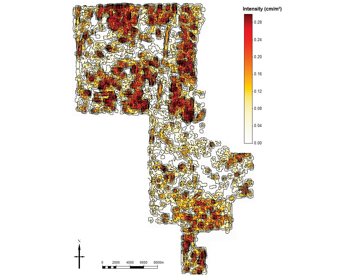
Fault intensity is calculated from an analysis of the directly-observed and inferred seismic-scale discontinuities, as detailed by Reine & Dunphy (2011). In map view, these faults are modelled as linear features, which allows for measurements of azimuth, length, and intensity (cumulative length per unit area). The intensity calculations are made over a 500 m x 500 m cell, which rolls in increments of 100 m (Figure 1).

Mechanical properties are obtained from a simultaneous AVO inversion (Hampson et al., 2005). The seismic data are first separated into four partial-angle stacks using the migration velocities. Residual moveout and amplitude balancing are then applied prior to the inversion. The inversion yields values of P-impedance, S-impedance, and density, which are then combined to produce volumes of Young’s modulus and Poisson’s ratio. The brittleness index B, is finally quantified using the Rickman et al. (2008) relationship

where E and v are Young’s modulus and Poisson’s ratio respectively, and the minimum and maximum values of these parameters are taken from the zone being characterized.

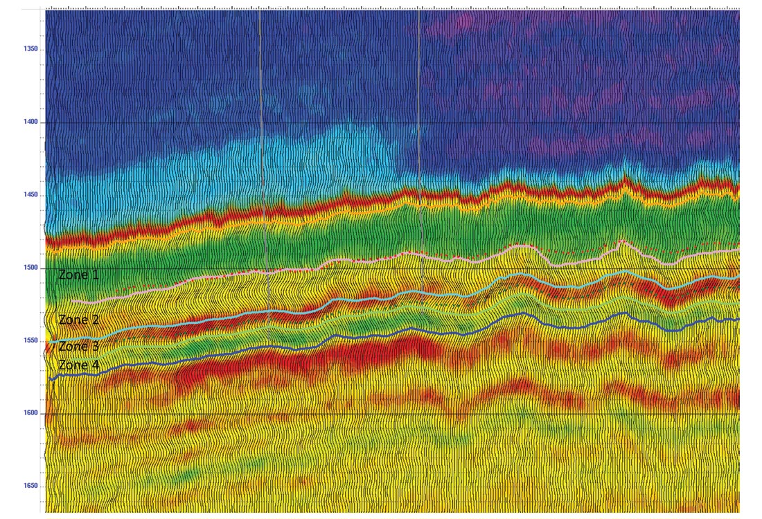
Four mechanical layers are seen in the data that correspond to geological boundaries (Figure 2). Using a 3D geological model, we first convert the geological layers into time, and then adjust them to the transitions between mechanical layers on the Poisson’s ratio volume. This allows for representative values in each geologically meaningful layer to be calculated and mapped.

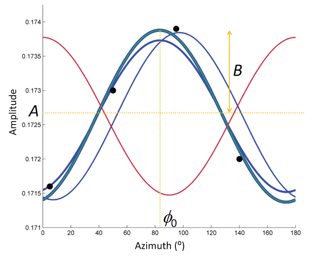
The same initial model and inversion parameters used for the above data are then applied to an inversion of gathers processed into four azimuthal sectors, this time with incidence angles restricted to 27º due to data limitations. Once mechanical properties are calculated, a function of the form

is fit to the median maps z of the inverted properties for each azimuth ɸ (Figure 3). This is an empirical fit following Mallick et al. (1998) and Lynn et al. (2010), which employs a non-linear inversion using the Gauss- Newton method (Aster et al., 2005). The background value A is checked with the full-azimuth inversion results for consistency. The ellipticity B provides a measure of the magnitude of azimuthal anisotropy, along with dominant direction ɸ₀. Poisson’s ratio shows a mean azimuthal anisotropy of 5% in each of the reservoir layers, and the mapped values are nearly identical to those of P-impedance. Because P-impedance requires a smaller range of incidence angles for accurate calculation, it is the more stable property and is therefore used henceforth.

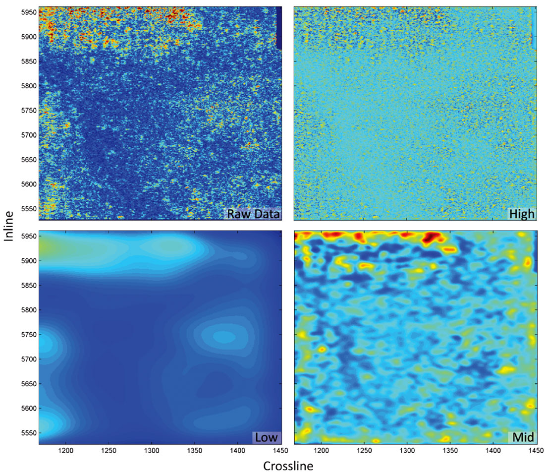
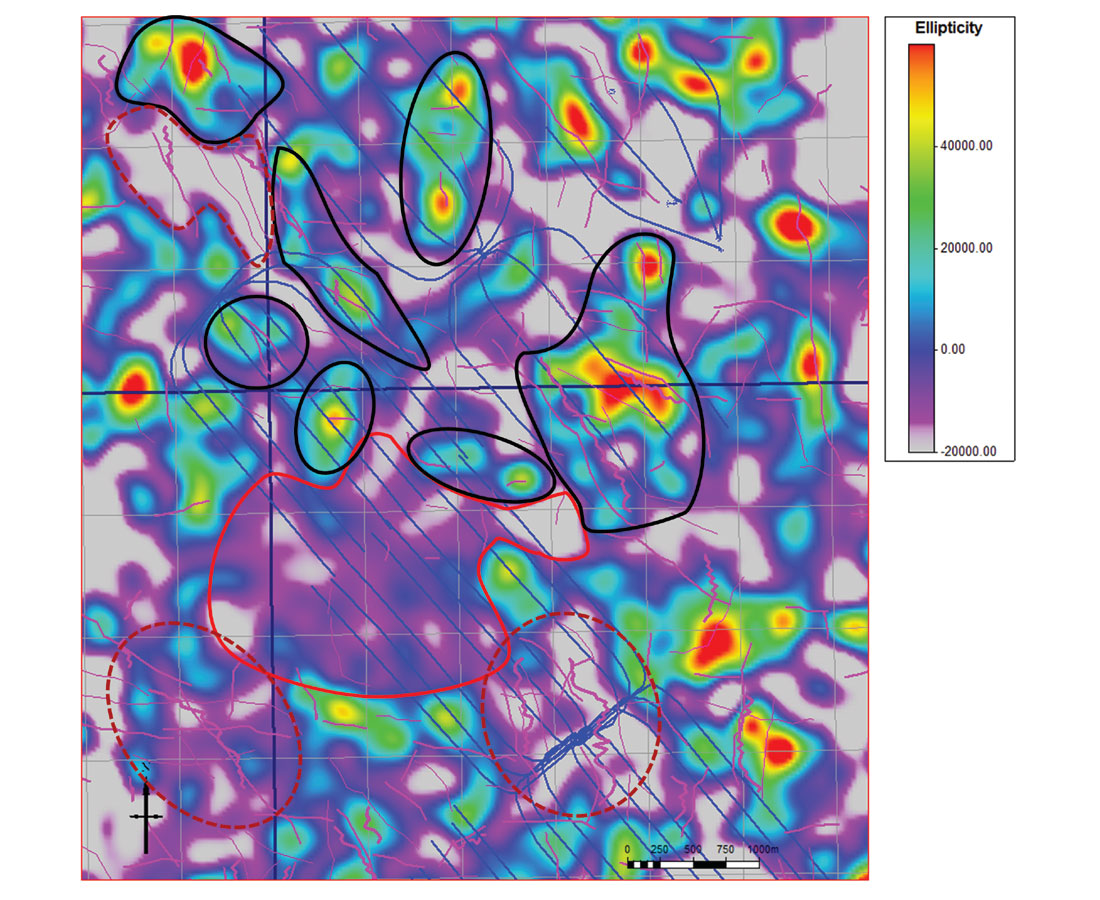
In addition to large and small-scale trends, the maps of ellipticity show a fair amount of high-frequency noise. This can be addressed by using a weighting function in the inversion, for example by inputting mean values of a 5x5 CDP area weighted by variance, or introducing spatial constraints. We find that a third option, spatially filtering the results, produces maps very similar to a weighted inversion, but with the added advantage of allowing the maps to be decomposed into high-, mid-, and low-frequency components (Figure 4). High frequencies are eliminated with a Gaussian low-pass filter. This filter is designed to have minimal reduction in amplitude for wavelengths at the average fault length of 577 m. In addition to the fault-scale variations in ellipticity, there are also more regional-scale trends that we hypothesize are due to regional stress variations. To isolate the fault effects, we design a second filter that significantly attenuates wavelengths smaller than 5 000 m, and subtract these low-frequency results from the previously filtered data.

Microseismic data was recorded for the hydraulic fracturing of 75 stages of a nine-well pad. The data consist of 93 725 events that include spatial, temporal, and magnitude attributes, among others. SRVs are calculated for each stage based on the event density. The SRV is nearly constant when increasing the percentage of points included from 30% – 70%. After this point, the SRV must increase substantially in order to accommodate a small number of outliers, which often are residual events from previous stages. For this reason, our SRVs use around 70% of the total points in a stage.

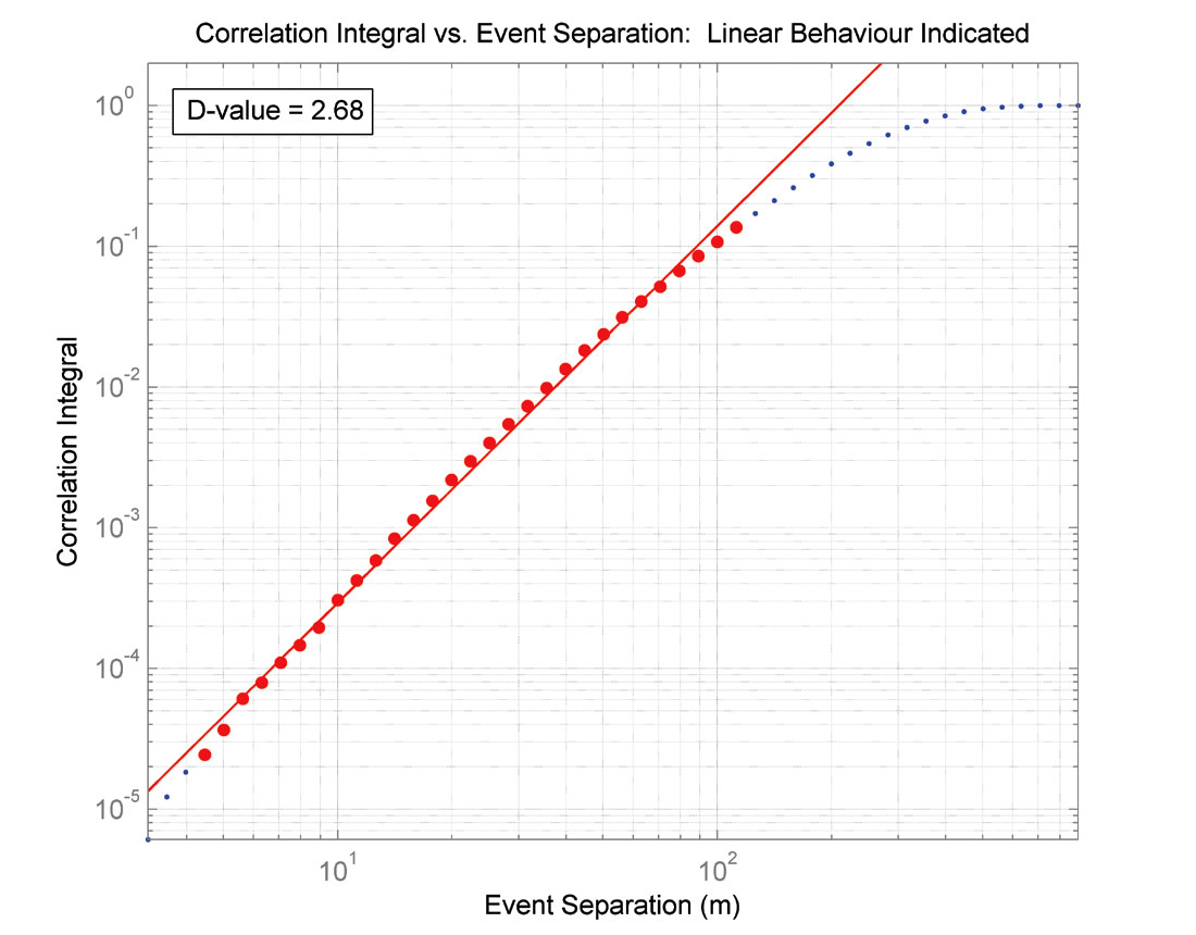
To characterize the data spatially, the ratio of SRV length to width, and the calculated D-value were both used. D-values are found by first determining the separation between each pair of microseismic events. The cumulative distribution of events N_r at a given separation r or smaller is used to calculate the correlation sum C

where N is the total number of events. The correlation sum is plotted versus the event separation in log-log space, and the D-value D is found from the slope of the linear region based on the relationship

where A is a proportionality constant (Figure 5).

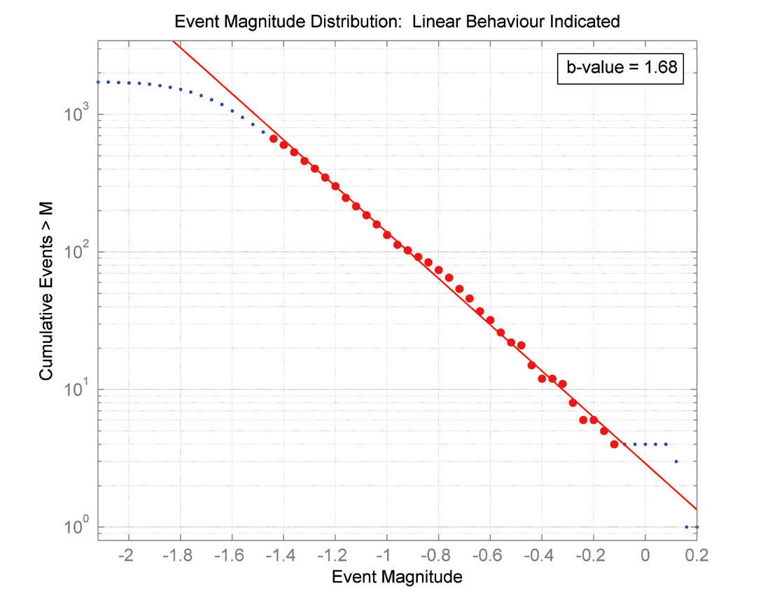
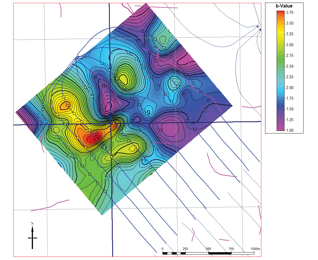
The microseismic b-value is determined in a similar manner for each stage in order to characterize the magnitude behaviour. The logarithm of the cumulative number of events N_M greater than or equal to a given magnitude M is plotted versus magnitude. The b-value is found from the slope of the linear region based on the relationship

where a is a proportionality constant (Figure 6).

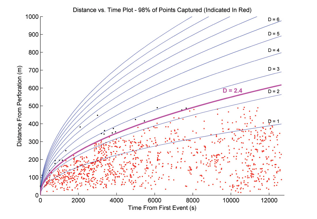
Finally, hydraulic diffusivity is calculated from the envelope of events on a distance to perf. versus time graph, with the intention of describing the velocity of fluid propagation. The distance r_p between the perf. and microseismic event is calculated and plotted versus time t. A diffusivity value D_H is calculated from the functional relationship that describes the envelope of the plotted points (Figure 7). The value for D_H is chosen so that the maximum number of points are included with only small incremental increases in D_H.

Analysis

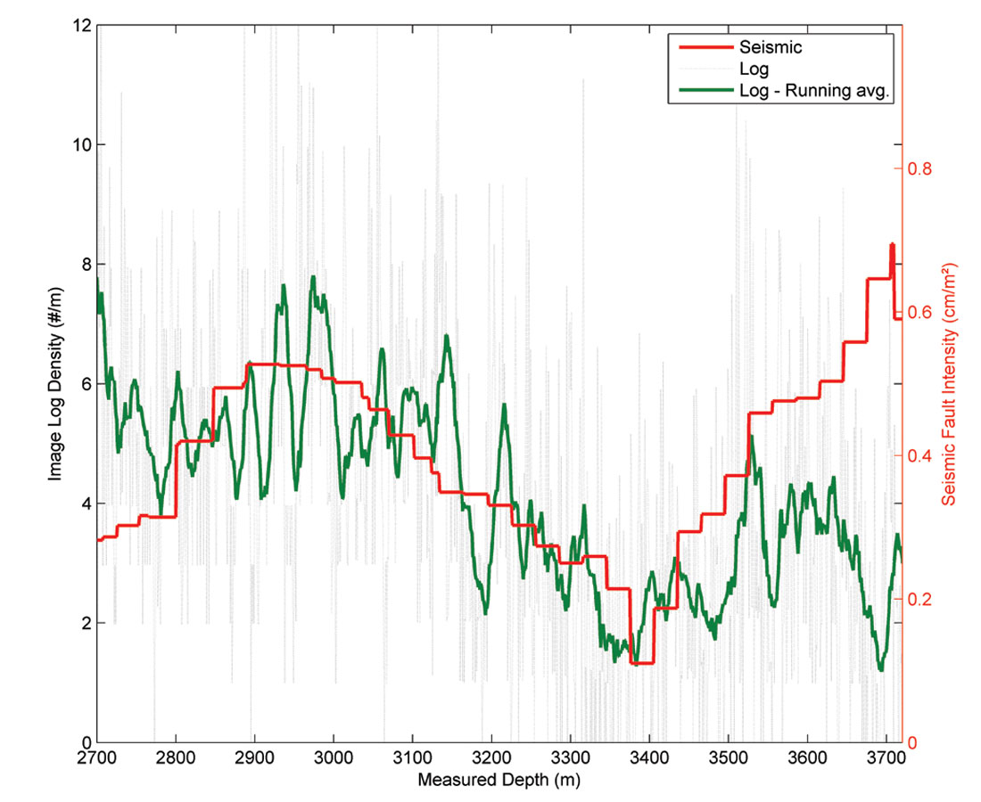
The relevance of seismic-scale faults is that natural fractures are expected to display a predictable scale relationship, often a power-law, between large and small features (Bonnet et al., 2001). The smaller microseismic failure radii, calculated using a Brune model (Brune, 1970), align with the same scale relationship as determined by seismic faults. This is consistent with the idea that hydraulic fractures, and the microseismic events that they cause, occur largely by reactivation of natural features. The calculated fault intensity is closely correlated to the fracture count from an FMI log in a horizontal well, supporting the assumption that large-scale faults are associated with an increase in small-scale fracturing (Figure 8).

The seismically observed faults also show a reasonable correspondence with azimuthal anisotropy. Figure 9 shows the mid-frequencies of the P-impedance ellipticity in zone 4. Numerous examples are seen where high ellipticity is associated with high fault intensity and typically these faults are in a single direction. Conversely, low ellipticity is seen in areas with low fault intensity. A third situation arises showing the breakdown of the method employed. Areas of low anisotropy are also seen in some areas with high fault intensity; however these faults tend to be in multiple directions. This is an artifact caused by restricting our analysis to four sectors of data, whereby it is not possible to identify multiple orthogonal fracture sets. This situation would require a more rapidly varying function than that given in equation 2. Nevertheless, approximately 75% of the data fit the cos2φ model with reasonable uncertainty.

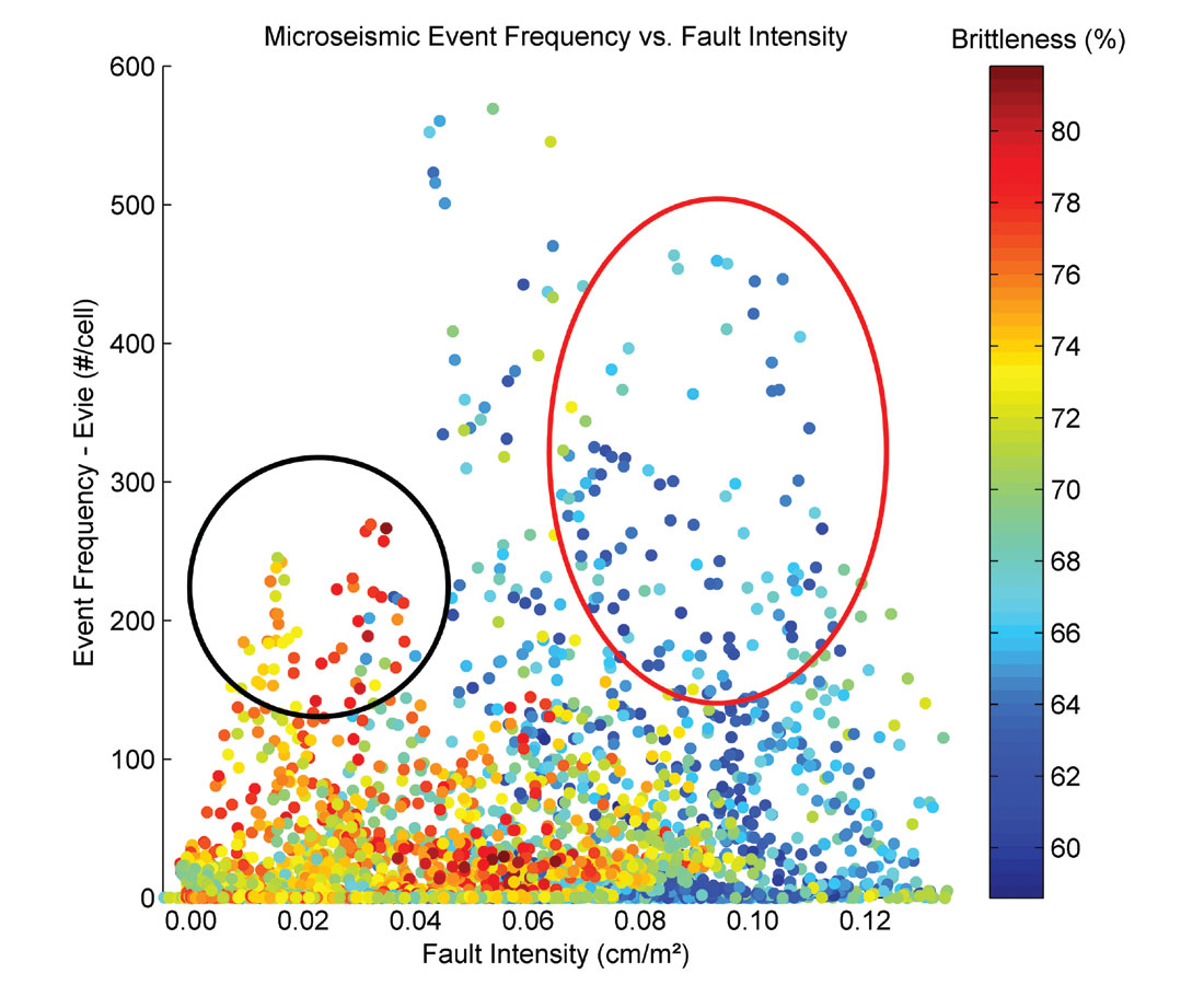
However fault intensity, which here is based on the ability to resolve (or at least infer resolution of) discontinuities, does not completely characterize a reservoir. The mechanical properties of the rock are also an important factor. Figure 10 shows a plot of microseismic event density versus seismic fault intensity, with points coloured by brittleness. These data are specific to a single geomechanical zone in the reservoir. Two peaks in event frequency can be seen, the first corresponding to the highest fault intensity. The second peak, while at a lower fault intensity, has the highest brittleness values, showing that both factors control the location of microseismic events.

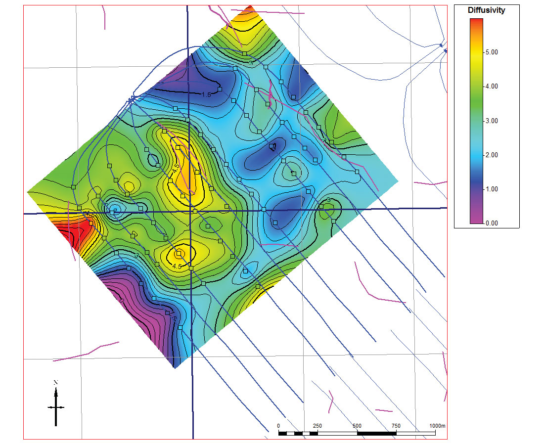
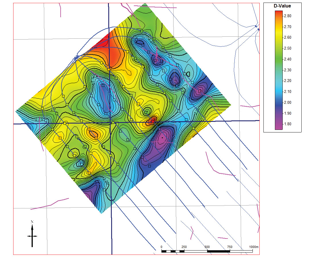
The spatial dimensions and kinematics of the microseismic clouds are also affected by fault intensity. The ratio of SRV length to width for stages adjacent to faulted areas is higher than for unfaulted areas. This indicates that the events are able to travel further away from the well in these faulted areas. Similarly, the hydraulic diffusivity in faulted areas is larger than in unfaulted areas, showing that the fluid front is able to move rapidly through the fault network (Figure 11). This is also true when only the z-component diffusivity is considered, indicating that fluid flows more easily in the vertical direction when faults are present. The microseismic D-values also indicate that frac behaviour is different when faulting is present. D-values are uniformly lower (D≈2) in faulted areas (Figure 12), suggesting behaviour that is more planar in nature. Larger D-values in areas without faulting indicate that the microseismic events are more uniformly distributed.

The distribution of event magnitudes are also affected by the presence of faulting, showing that there are likely changes in the failure mechanisms. In regions where faults are present, we consistently observe lower b-values (b≈1), suggesting that these events are dominated by hydraulically-induced reactivation of natural-fault networks as suggested by Maxwell et al. (2009) (Figure 13).

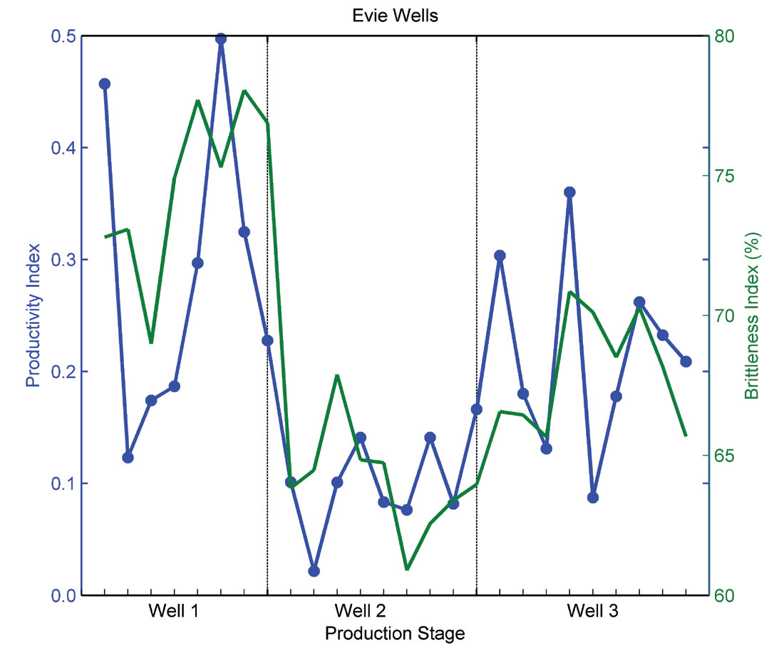
While microseismic data indicate the quality and extent of the hydraulic fracture operations, the ultimate key indicator is well production. Production logging was carried out on seven horizontal wells, giving information on 53 stages in the uppermost reservoir zone (zone 1) and 26 stages in the lowermost reservoir zone (zone 4). A productivity index is calculated which allows the comparison of stage contributions across multiple wells. We find that the major influencing factors in productivity vary by reservoir zone.

For zone 4, a strong correlation is seen between the productivity index and brittleness (Figure 14). This is echoed by the overall well production results which show the highest zone 4 producers occurring in high brittleness areas. In zone 1 however, the brittleness is less of an influencing factor. In this zone, there is a moderate correlation with the mid-frequency P-impedance ellipticity. A possible explanation for this lies in the observation that the range of brittleness in zone 1 is less than half of that in zone 4. This indicates that brittleness would be less of a factor since it is more uniform, and the production is more closely tied to the natural fracture network.

Conclusion

Predicting the behaviour of a shale-gas reservoir is an ambitious goal with great value. While we are not suggesting that seismic data alone is able to provide all of the necessary characterization, we have shown that some valuable information is nevertheless available. By observing the seismic-scale faults on the seismic image, and by calculating the reservoir’s mechanical properties through AVO inversion, we are able to validate observations from microseismic and production data.

In our examples, hydraulic fractures tend to produce the most microseismic energy in areas with high fault intensity, followed closely by areas with high brittleness. The natural faults affect the spatial distribution of the microseismic cloud and how fast the fluid front propagates, causing the events to move further and faster away from the well. The analysis also indicates that microseismic events in faulted areas are reactivation features, having shapes that are more confined to a plane, magnitude distributions that are more like natural seismicity, and having length distributions consistent with natural features. Finally, while gas production is a complicated process, the highest gas production for the lowest zone wells comes from areas with higher brittleness, while for the upper zone wells, production increases with higher azimuthal anisotropy.

Acknowledgements

A large number of people have been involved in the everyday operations that have contributed to this work, from data collection and processing to geological modelling and production analysis. We would like to thank Nexen’s shale gas team for their efforts, and thank Nexen for allowing us to show these results.