Estimating the value of Geophysics: decision analysis

Summary

This paper discusses the value of geophysical data in the resource play paradigm. Specifically, it shows how well known decision analysis techniques can be applied to estimate the value of seismic for resource play examples. We examine the sensitivity to the accuracy of the seismic interpretation and to the spread of expected values of the drilling being considered. The results are strongly supportive of the investment of the seismic under certain conditions. Sensitivity to seismic reliability also implies economic support to low cost efforts such as processing that may increase the reliability of the interpretation. Even under conditions where the initial economic success of the wells is as high as 75% to 80%, and the seismic data only adds a small additional advantage, it can be strongly economic to buy and use the seismic data. This argument for the value of seismic is practical, conservative, and reasonable because it recognizes seismic as imperfect information through the use of Bayes’ Theorem. The use of decision analysis techniques, including sophisticated techniques such as Bayes’ Theorem, is of particular use because the results are manifest in the language of engineers; that is in the form of decision trees, statistics, and expected value.

The question of the value of seismic is topical. The oil and gas resource business environment has changed, particularly in the perception and economic meaning of risk. Risk has always been a short form for describing the probability of various desirable or undesirable outcomes, and in the resource play environment we have vastly reduced the probability of not encountering reservoir or hydrocarbons. Somehow this change in conditions has led many to incorrectly assume that there no longer exists a spectrum of outcomes with associated desirability. Even in resource plays there is commonly a significant variation in the flow rates, ultimate recoveries, and values of individual wells. The value of seismic in these new resource plays is dependent on the probability distribution of and economic differences in the spectrum of outcomes available. We will show that if we understand these probabilities and their economic differences, we can quickly assess how valuable seismic data is.

Introduction

Geophysical data and its interpretation should only be invested in if it has value to the investor. This is no surprise; we should not invest in anything that lacks a value argument, otherwise it is charity. We do not perform geophysics for intrinsic reasons; in business we have no interest in it as a thing in itself. The value of geophysical data may be estimated in a variety of ways, none of which are materially different from the way of determining the value of other kinds of information such as log data. We shall briefly discuss the case study method of determining the value of geophysical data, but we will spend more time on the decision analysis method of estimating the value of seismic data. The decision analysis approach is often overlooked for many reasons. Some people overlook the method because they do not understand how to handle the imperfect nature of seismic. We will address that with Bayes’ Theorem. Some geoscientists and engineers are fond of suggesting they can just “high level” (or guess) the decision, which may be because they have already gone through the decision analysis technique exhaustively, but is more often a pococurante excuse to avoid trying anything. Many others do not use decision analysis because they have a hesitancy to commit to a single set of parameters for the study. We will use sensitivity analysis to mitigate the problem of committing to only one set of parameters. Sensitivity analysis is essential to achieving sufficient understanding of a question so that the act of “high levelling” the problem becomes rational and reasonable.

The resource play framework, as created by our cousins in engineering, carries the explicit conditions that our drilling will encounter productive reservoir whose production behavior is statistically describable in an area. These explicit conditions clearly allow for some variation in productive capability, and further imply that we have some statistical description of that variation. Since the natural world universally contains variation, this allowance and implication is fundamental to the reductionist resource play concept being considered as reasonable. The economic value of investing in information such as seismic data therefore is heavily dependent on the magnitude of the statistical variation in well productivity and the seismic data’s probability of correctly predicting these variations in outcome.

Case studies

The value of geophysical data may be estimated from observation, but only if we have knowledge of sufficiently similar decisions being made with and without the information, together with an accurate description of the economic differences in the results. This observation, or case study-based approach requires the data be adequately controlled; that is, the only variable being changed is the effect of information. This requirement is heavy. Hunt et al (2012), showed the value of seismic versus no seismic and even the value of a new seismic processing technique versus an old seismic technique in the Viking play in West Central Alberta. The valuation of the processing technique in the Viking case specifically measures the economic effect of the reliability of the seismic data, and is unusual in the literature. The work required statistics from 69 different wells from which the knowledge of the Viking reservoir parameters and state of pre-drill geophysical effort was accurate. The results showed seismic related net present value (NPV) differences on the order of a million dollars per well as measured by differences in reservoir bulk storage and their associated rates, estimated ultimate recoveries, and decline analysis. Hunt et al (2012) also showed that improved steering accuracy generated economic improvements as measured by modeled barrels of oil per day in a Saskatchewan and Manitoba Devonian horizontal oil play.

The case study method of estimating the value of seismic is very important, and typically straight forward to understand. Gray (2011) cites other case study based examples, and the annual CSEG Symposium typically contains several value oriented case studies. What do we do when we do not have an applicable case study to refer to, but instead a new investment decision to make? What do we do when we are challenged to comment on how much we can or should spend on seismic in an area?

Decision analysis

Decision analysis is the science of formal decision making, and was developed in the 1960’s and 1970’s. Newendorp (1975) summarizes the science of decision analysis in an appropriate form for our discussion on the value of seismic data. Decision analysis uses tools of logic, and considers multiple possibilities arising from choices or decisions. Typically, the best decisions in petroleum business have the best economic outcomes, although preferences may also be considered. A key aspect of oil and gas decision analysis is the explicit handling of uncertainty and imperfect information. The inclusion of uncertainty and imperfect information require the analysis to include not only choice milestones, but also chance or probability milestones. A key tool in decision analysis is the decision tree, wherein the decision milestones are called decision nodes (represented as squares) and the chance or probability milestones are called chance nodes (represented as circles). Decision trees are solved backwards towards the time zero beginning. The imperfect nature of seismic information requires us to use Bayes’ theorem in our handling of probability in our decision analysis.

Newendorp’s method: Bayesian decision analysis

Newendorp (1975) describes a general approach that may be used to estimate the value of any imperfect information prior the point of making a decision that has uncertainty. Geophysical information belongs to a large class of knowledge coined by Newendorp as “imperfect information” because it is subject to multiple interpretations, and does not precisely tell us the true state of nature. The uncertainty or imperfection of this knowledge necessitates the use of conditional probability, usually in the form of Bayes’ Theorem within the decision tree structure of Newendorp’s method. The method requires some estimate of the probability (reliability) of the interpretation from the imperfect information, the possible states of nature described by the work and the expected values of all possible outcomes. The original, or initial, probability of each possible outcome is also an important aspect of this analysis. This initial information and its accuracy can sometimes be a cause for controversy, as it has an impact on the final revised probabilities being considered. In the examples that follow, consider carefully the original probabilities we use.

Bayes’ Theorem, defining the probability of any event Ei given the interpretation, B, is:

Let us explain this further.The original, initial, or absolute probabilities, are P(E_i), which come from prior knowledge. These are the likelihood of each of the E_i events occurring.

The information that we bring in (say geophysical data such as seismic) defines event B. In the case of seismic, B might be an interpretation from the data that a channel is present. The reliability of the information indicating event B is given as P(B|Ei). This is the probability, accuracy, or reliability of the interpreted information being correct.

Bayes’ theorem is useful because it combines the reliability of the information with the original probabilities of each event. The solutions to Bayes’ theorem, P(E_i|B) may be thought of as a new or revised probability of occurrence for event E_i, given the information B, and the original probability P(E_i).

The “probability of the interpretation” and the expected values of the outcomes are key measures that may also be understood as the observed data in the case study or observation based method we discussed earlier. Geophysicists can add value best by focusing on information or efforts that improve the reliability of their interpretation of reservoir quality, or by applying the imperfect information to problems with the greatest variation in expected values. Timing of effort is also important: since reservoir uncertainty is the largest early in a project, geophysical data has the greatest impact then. This has long been intuitively understood, which is why geophysical data has been most frequently used in exploration. The high capital nature of resource plays often make geophysical data of economic benefit throughout the life of projects.

Example: Mannville channel well and seismic

A decision is being contemplated as to drill a well into a welldefined, thick, and broad, Mannville channel system in West Central Alberta. The well costs $5,000,000 to drill, complete, and tie-in or $3,000,000 to drill alone. There are several choices of well positioning available. If this decision well is not drilled, another location will be picked. There are two possible (states of nature) outcomes for the well’s production and consequent present value: the well misses the channel system, or the well encounters the channel system and hits statistically average rock for the system. The stabilized initial rates (excluding liquids) and present value of these states of nature are:

1. Misses the channel: 0 mmcf/d, $0 present value (PV)
2. Average well: 4mmcf/d plus liquids, $6,500,000 PV

The probabilities of encountering each of these states using existing well control are: 0.2, 0.8, respectively. That is, there is an 80% chance that any given location on the land will encounter the channel system.

The company is contemplating buying trade seismic data over the area. The seismic will change the perceived risk of the well, and perhaps determine whether this well is drilled or is set aside in favor of other locations. The seismic costs $100,000 for every well being examined. Using the seismic data, any of the two states may be interpreted: first that the well being proposed will encounter channel sand, or secondly that the well will not encounter channel sands. The probability of the interpretation being correct in either case is 0.9. That is, there is a 90% chance that the well will encounter the geology predicted by the seismic.

There are two broad strategies that can be employed: the first being the so-called “gamble strategy” where we choose to drill the well without seismic. Given the high chance (80%) of encountering the channel, this approach may be tempting, and many operators would choose it. The play is in fact being treated as if it were a resource play where reservoir is locally guaranteed. This is not actually correct, but the high chance of success is driving perception. The second strategy is to acquire the seismic for a cost of $100,000 per well decision. The seismic itself is uncertain or imperfect information. Within the seismic strategy, there is also the possibility to ignore the seismic interpretation. This could be influenced by the high initial probability of encountering channel or by land, pipe, or surface conditions. In describing the best decision, and the value of the seismic strategy, we will use Newendorp’s method. We will refer to Chart 1, the decision tree throughout the analysis.

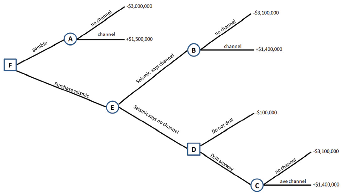
In Chart 1, we see that we have several choices: first, at decision node F we choose to either gamble and drill using our original estimate of probabilities, or do we choose to purchase the seismic. If we purchase the seismic, we come to chance node E where the seismic may yield an interpretation that the well location will encounter channel, or the interpretation may be that the well will miss the channel. Node B follows the “interpreted channel” probability and explores the possibility that the well either encounters channel or it does not. Decision node D follows the “interpreted no channel” branch and explores the possibility that a decision is then made to either not drill the well, or to drill the well. Chance node C explores the possibility that despite the “interpreted no channel” outcome from the seismic, the decision was made to drill the well anyway. The NPV for each outcome is given. But which of the decisions yield the highest expected NPV? Should we gamble or acquire the seismic? If we have the seismic, should we accept the interpreter’s advice? The answers to these questions use Bayes’ Theorem as Newendorp explained.

Let us first define the events and probabilities succinctly:

E₁ = event or state of nature 1 = the channel will not be present

E₂ = event or state of nature 2 = the channel will be present

The original estimated probabilities are:

P(E₁) = original estimate that channel will not be present = 0.20

P(E₂) = original estimate that channel will be present = 0.80

The outcomes from the seismic interpretation are:

B = the seismic suggests the channel will be present, B’ = the seismic indicates the channel will not be present

The conditional probabilities of the seismic interpretation B given the states of nature:

P(B|E₁) = 0.1 = probability that the seismic says there is a channel present when there is in fact not a channel present.

P(B|E₂) = 0.9= probability that the seismic says there is a channel present when there is in fact a channel present.

The B’ seismic interpretation probabilities are simply interchanged with the B probabilities.

If we are going to evaluate the decision tree, we must remember Bayes’ Theorem, defining the probability of any event Ei given the interpretation, B, which is given by equation (1).

Let us work through the solutions to Bayes’ theorem for the two interpreted seismic cases corresponding to each of the two events we defined; that our interpretation could indicate a channel, or that there is no channel where we wish to drill the well.

Table 1 shows the solution to Bayes’ theorem if B indicates a channel. Column three in Table 1 shows the calculation of the numerator of Bayes’ Theorem. These values arise from the multiplication of the values from columns one and two. We also call these probabilities the Joint probabilities. The joint probabilities sum to 0.74, which is the denominator of Bayes’ Theorem, and is the total probability that the seismic interpretation will suggest a channel will be encountered. Column four in Table 1 shows the solution to Bayes’ theorem, and is thus each value in column three divided by the sum of column three. The solution to Bayes’ theorem is also called the revised probabilities or revised risk estimates of each event given the interpretation.

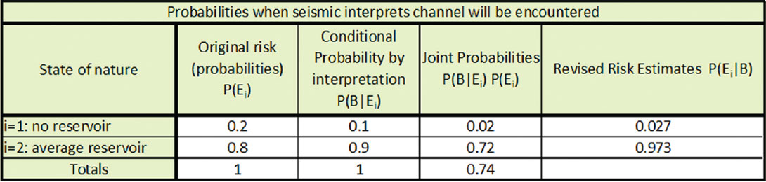
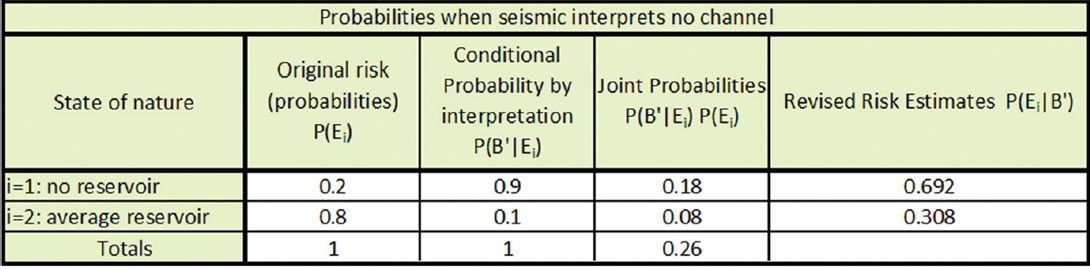
Table 2 shows the solution to Bayes’ theorem if B’ indicates there is no channel at the well location. Column three in Table 2 shows the calculation of the numerator of Bayes’ Theorem. Just as was the case for interpretation event B in table 1, this is the result of the multiplication of the values from columns one and two. These joint probabilities sum to 0.26, which is the denominator of Bayes’ Theorem, and is the total probability that the seismic interpretation will suggest a channel will not be encountered. Column four in Table 2 shows the solution to Bayes’ theorem, and is thus each value in column three divided by the sum of column three.

Now we have all the probabilities we need to solve the decision tree. Chart 2 illustrates the decision tree with the probabilities and expected values filled in. Let us go through the solution at each node.

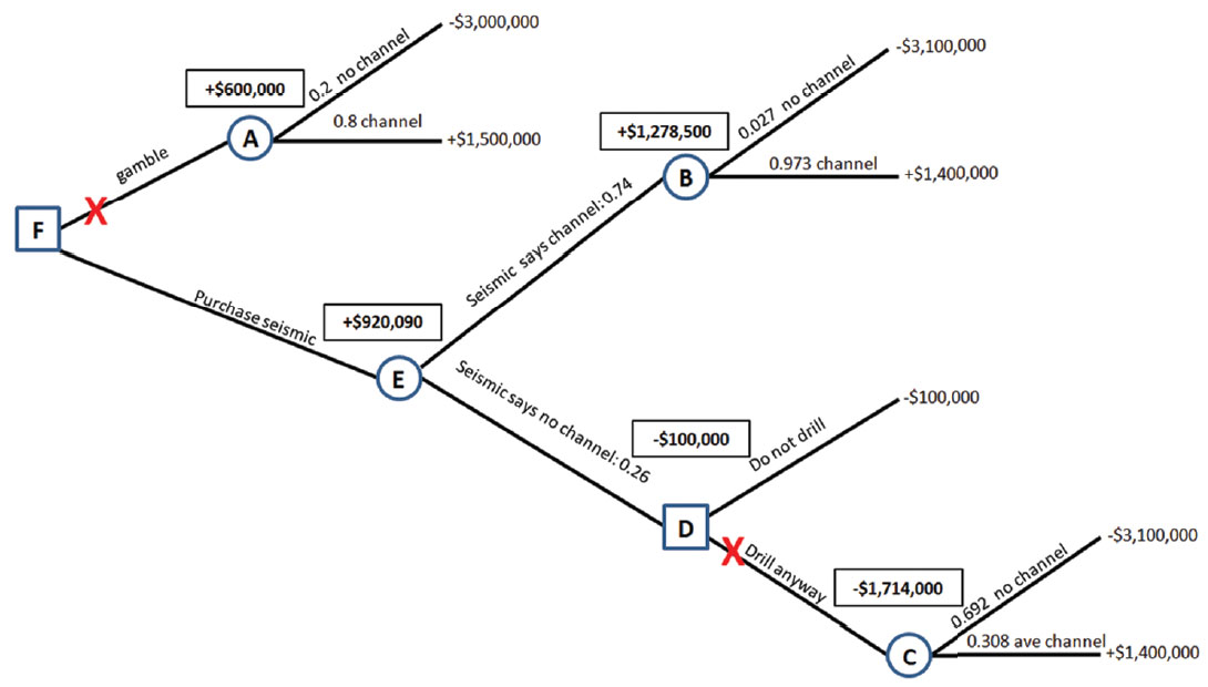
The expected NPV at node A, the choice to gamble, is simple. It is:

NPV (E₁) * P(E₁) + NPV (E₂) * P(E₂) = -$3,000,000 * 0.20 + $1,500,000 * 0.80 = +$600,000.

The expected NPV at chance node B, where the seismic interprets there will be a channel is:

NPV (E₁) * P(E₁|B) + NPV (E₂) * P(E₂|B) = 0.027*(-$3,100,000) + 0.973*(+$1,400,000) = +$1,278,500.

The chance that we ever get to node B from node E and enjoy this positive NPV is 0.74, or the numerator of Bayes’ Theorem.

The expected NPV at chance node C, where the seismic interprets there will be not a channel, and we still drill the well is:

NPV (E₁) * P(E₁|B’) + NPV (E₂) * P(E₂|B’) = 0.692*(-$3,100,000) + 0.308*(+$1,400,000) = -$1,714,000.

The chance that we ever get to choose to go to node C from node D and E and enjoy this horribly negative NPV is 0.26. The choice to drill when the seismic interpretation suggests there will be no channel is thus seen as strongly uneconomic.

Let us now look at node D. This path comes about if the seismic interpretation, E, suggests there will be no channel. In such a case, we may choose at node D, to not drill a well. This would give us a NPV of -$100,000, which was the value of the seismic. Deciding not to drill rather and lose $100,000 is a much better decision than to drill and lose $1,714,000. This means the no channel interpretation is now understood to mean no well is drilled, yielding an NPV of -$100,000.

So, what is the overall expected value of the seismic, and should we purchase it? The expected value of the seismic is the chance the seismic would interpret channel multiplied by the expected value of the subsequent branch plus the chance the seismic would interpret no channel multiplied by the expected value of the subsequent branch. This is the expected value at node E:

0.74 * $1,278,500 + 0.26 * (-$100,00) = +$920,090.

Note that the branch weights are the denominators of Bayes’ theorem for each interpreted case.

Therefore, for each contemplated well, the NPV is +$920,090 with seismic or +$600,000 without it. The decision tree is filled in with all of this data in Chart 2.

This suggests that the seismic should be used. The value of the seismic is much higher than its expense. Moreover, this is a per well value, so the project value of the seismic will be much higher. Sensitivity analysis of the seismic reliability and cost can be performed with this method, which could determine the maximum amount that should be spent on seismic, or the minimum change in the probability of success that the seismic can afford while still enjoying an advantage in expected value.

Example II: resource play quality

Let us look at another example involving a true resource play. This play is more expensive with drill, case, complete, equip, and tie-in costs of $6,000,000. The target is pervasive, and all wells that are drilled will be completed. This play is developed on a four horizontal wells per section basis, and there is some flexibility in drill order. Usually, development happens by surface pad and section (hub), which means there is a cost efficiency associated with fully developing (drilling four wells per section or pad) each hub at one time or in sequence. Therefore, there is an economic penalty to deferring drilling a well within a pad when the rest of the pad is being developed. This cost is minor, but fully accountable, and is $100,000 per well deferred.

The event outcomes for drilling have been studied and are reasonably well known. The events are:

E₁ = poor producing well. NPV = -$2,500,000

E₂ = average producing well. NPV = +$1,500,000

E₃ = superior producing well. NPV = +$5,000,000

The well understood, initial, probabilities of each of these outcomes are: P(E₁), P(E₂), P(E₃), which are 0.25 for a poor well, 0.50 for an average well, and 0.25 for a superior well.

Seismic could be shot and processed for a cost that works out to be $50,000 per well location. Seismic discriminates the quality of the well locations through amplitude versus offset analysis (AVO) identification of superior reservoir quality and fracability (Goodway et al, 2006, Close et al, 2012). The seismic further discriminates the likely quality of the well by identifying undesirable stress regimes with azimuthal amplitude versus offset analysis and converted wave analysis of shear wave splitting (Close et al, 2012). The seismic reliability will be given a value of 0.90.

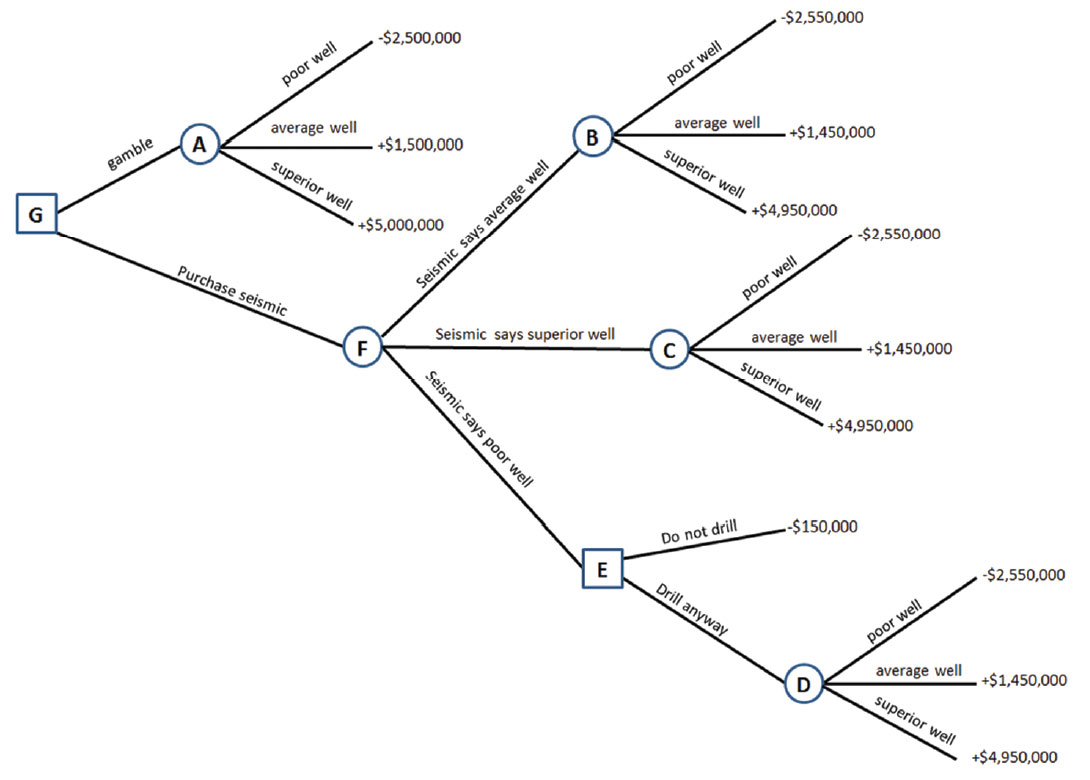
We can build a decision tree as we did in example I, to help guide us in this decision analysis. This decision tree is shown below in Chart 3.

Let us work through the solutions to Bayes’ theorem for the three interpreted seismic cases corresponding to each of the three events we defined; that our interpretation could indicate a poor well, and average well, or a superior well.

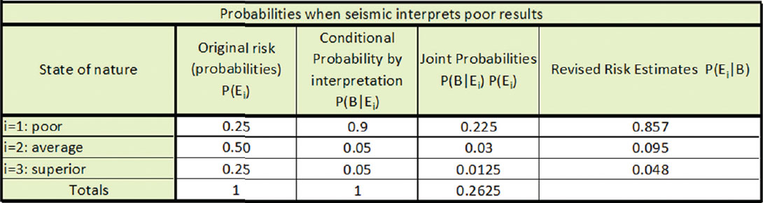
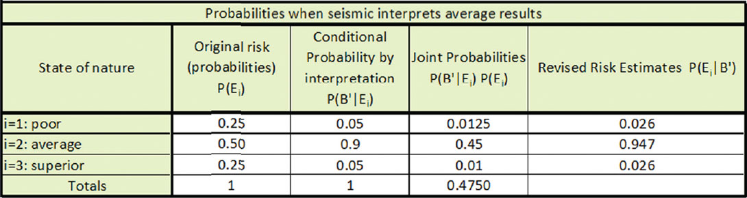
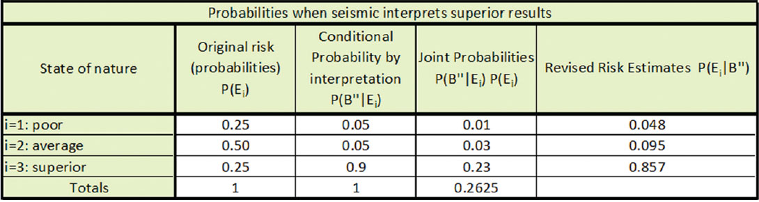
Table 3 shows the solution to Bayes’ theorem if B indicates a poor well. Table 4 below shows the solution to Bayes’ theorem if B’ indicates an average well. Table 5 below shows the solution to Bayes’ theorem if B’’ indicates a superior well. The revised probabilities are respectively similar for the poor and superior well interpretations, as we would expect them to be. The revised probability of the average well interpretation has the highest probability for any event, the average well event of 0.947, which we would also expect given the original probabilities.

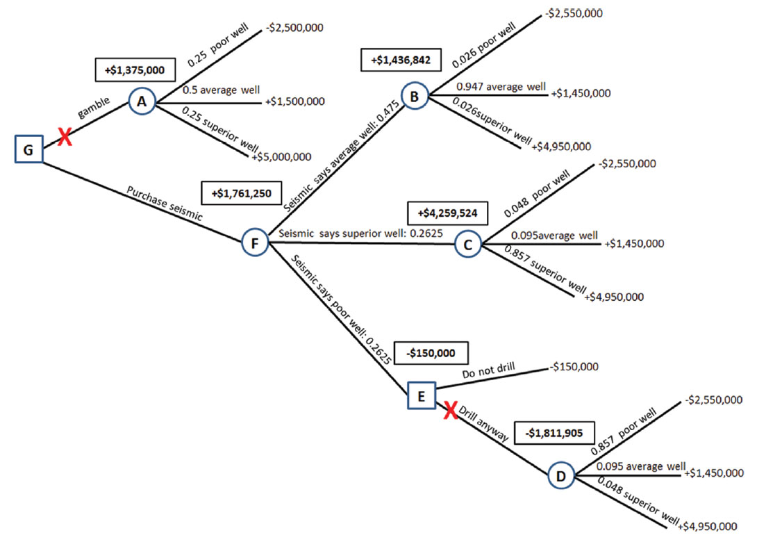
Now we have all the probabilities we need to solve the decision tree. Chart 4 illustrates the decision tree with the probabilities and expected values filled in. Let us go through the solution at each node.

The expected NPV at chance node A, the gamble scenario is:

= 0.25 * (-$2,500,000) + 0.5 (+ $1,500,000) + 0.25 * (+$5,000,000) = +$1,375,000.

The expected NPV at chance node B, the seismic interprets an average well is:

= 0.026 * (-$2,550,000) + 0.947 (+ $1,450,000) + 0.027 * (+$4,950,000) = +$1,436,842.

The expected NPV at chance node C, the seismic interprets a superior well is:

= 0.048 * (-$2,550,000) + 0.857 (+ $1,450,000) + 0.095 * (+$4,950,000) = +$4,259,524.

The expected NPV at chance node D, the seismic interprets a poor well is:

= 0.857 * (-$2,550,000) + 0.095 (+ $1,450,000) + 0.048 * (+$4,950,000) = - $1,811,905.

Decision node E becomes a choice of either -$1,811,905 from chance node D, or -$150,000 if the well is not drilled. The value of -$150,000 includes the - $50,000 cost of the seismic and the - $100,000 operational penalty from deferring to complete a surface pad in order. The decision is made to defer drilling the well.

The expected NPV at chance node F, the seismic interpretation is:

= 0.475 * chance node B + 0.2625 * chance node C + 0.2625 * decision node E = +$1,761,250.

This means that the purchase seismic decision yields a much higher expected NPV (+$1,761,250) than the gamble strategy, and is thus the choice made at decision node G.

Sensitivity to quality of seismic interpretation

We can create another version of the example II scenario where we consider the sensitivity of the results to the reliability of the imperfect seismic information. We can hold all other variables the same as in example II, except for the seismic reliability, and recalculate the expected values.

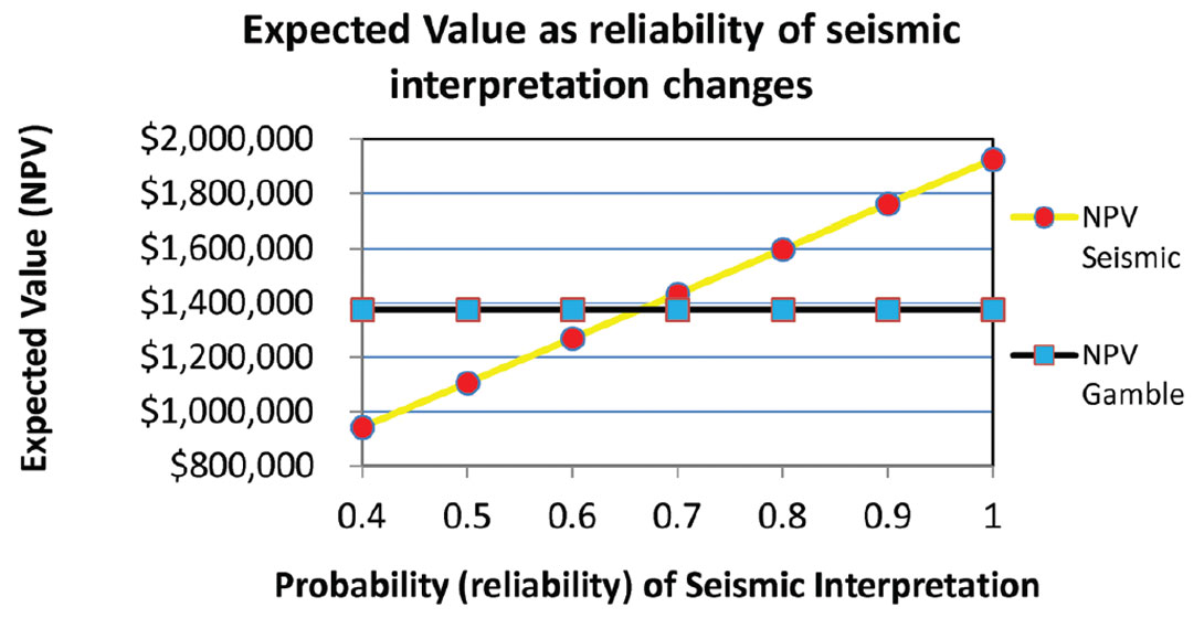
The seismic reliability will vary from 1.0 (perfect information) to 0.4. The results of this sensitivity analysis are illustrated in Figure 1. The gamble scenario expected values are invariant at +$1,375,000 as the seismic reliability changes. The seismic method expected values are shown by red circles, and change linearly with the reliability of the interpretation. The break even seismic reliability is just under 0.70. the maximum value of the seismic method, reached at perfect reliability, is +$1,925,000. At high reliabilities, the seismic method has significant value relative to the gamble scenario.

Sensitivity to poor well NPV

We can create another version of the example II scenario where we change the spread of NPV values associated with each case.

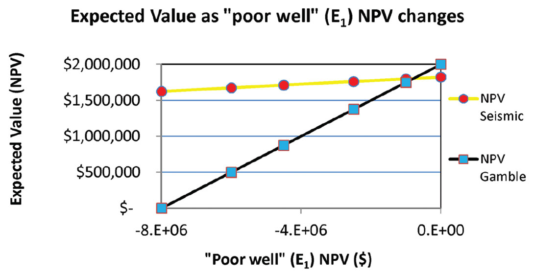
Specifically, we vary the expected value of the poor well or E₁ event and observe the effect this has on the expected value of the seismic method. The variation in the poor well event goes from an NPV of $0 to -$8,000,000. This worst case scenario could primarily come about if the well had unusual operational difficulties (in either drilling or completion, or both) and was not productive.

If we use the same decision tree structure as in example II, we can calculate the expected values for this scenario. Again, we have the gamble scenario versus the seismic scenario. Figure 2 illustrates the results graphically. The expected value of the gamble approach changes much more drastically than the expected value of the seismic approach. This is because the seismic information is purposefully used to avoid, within its reliability, the effect of the poor well. As a result, the expected value arising from the use of seismic is higher that the gamble approach through most of the graphed space. This is due to the low NPV range of the poor well scenario and the high reliability of the seismic. These cases show a significant value to the use of seismic.

Different conditions and sensitivity to reliability of seismic interpretation

We can create another version of the example II scenario where we change both initial probabilities and the spread of NPV values associated with each case. Given a change in these values, we can further explore the required reliability of the imperfect seismic information. In this example, the values of the initial events become:

E₁ = poor producing well. NPV = -$4,500,000

E₂ = average producing well. NPV = +$1,500,000

E₃ = superior producing well. NPV = +$5,000,000

The probabilities of these events are changed to: P(E₁), P(E₂), P(E₃), which are 0.175 for a poor well, 0.65 for an average well, and 0.175 for a superior well. This new scenario describes a resource play where the average outcome is much more likely than either of the other events, but that the poor event is more economically damaging as compared to example II.

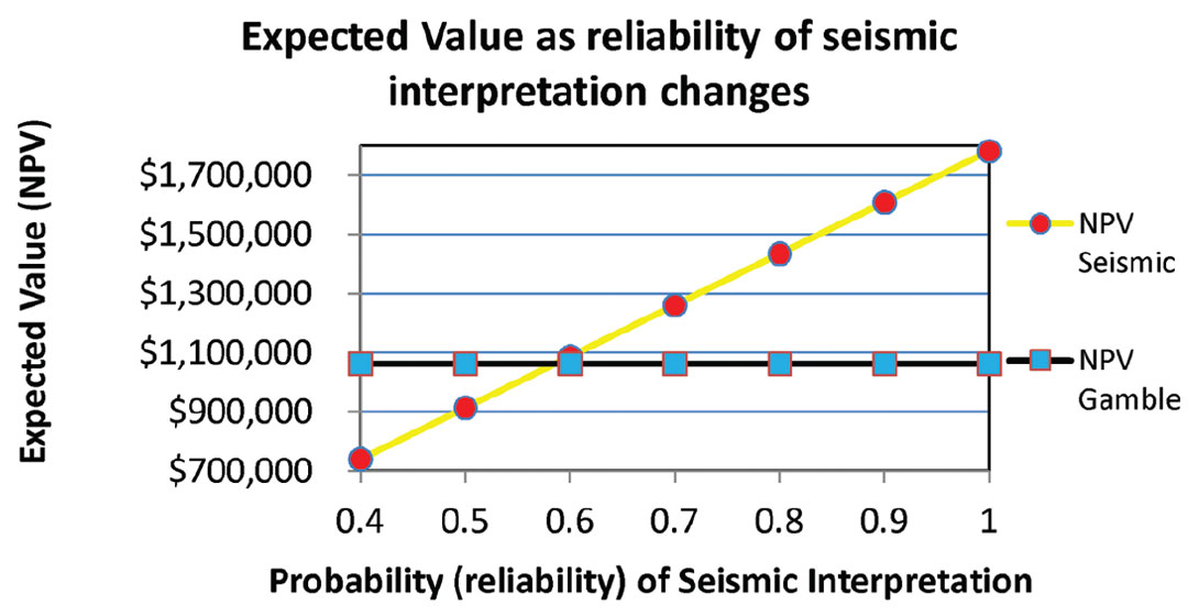
If we use the same decision tree structure as in example II, we can calculate the expected values for this scenario. Again, we have the gamble scenario versus the seismic scenario. We can evaluate the sensitivity of the economics to the reliability of the seismic by running our calculations for a variety of seismic probabilities, specifically from 1.0 or perfect reliability down to 0.4. Figure 3 illustrates the results graphically. The gamble scenario has an invariant expected value of +$1,062,500. The expected value when we use the seismic surpasses the gamble scenario prior to a reliability of 0.6, and has a maximum expected value of +$1,782,500 when it reaches perfect reliability. The seismic is thus more valuable in this example, mostly due to the fact that the poor well outcome is indeed quite economically damaging. The change in original probabilities was not as dominant as the change in poor well outcome.

Implications of the value of reliability

The sensitivity of expected value to the reliability of the seismic as shown in graphs 1 and 3 have broad implications to how we shoot and process seismic data. Since expected values always increase with increasing reliability, then increasing reliability is good business. The reliability of the seismic is subject to many factors including the quality of its processing, the effort and appropriateness of the acquisition parameters to the specific geologic target, and also to the interpretive techniques being employed. Some interpretive techniques require additional processing and investment. This means that there is objective economic motivation to invest in better processing, acquisition, and the use of the most advantageous interpretive techniques. Hunt et al’s (2012) Viking work demonstrated this principle explicitly on a real case. The limits of this investment could be studied further; however, in many cases the answers are obvious. Processing of seismic data is typically negligible compared to the costs being considered for the drilling and completion. This means that extra efforts in processing that increase the reliability of seismic are generally going to be worthwhile.

Conclusions

The meaning of risk in today’s world, is better expressed as the probability of a spectrum of results with different economic values. The use of Bayes’ Theorem makes the modeling of various economic scenarios reasonably straightforward even while recognizing that seismic is an imperfect kind of information. We showed a variety of examples in which sensitivity to the reliability of the seismic, initial probabilities, and variation in expected values were explored. The value of seismic is seen to be inextricably tied to its reliability and the degree of variation in the economic outcomes. A “high level” truism from this work is that the value of seismic can be very significant when it has a high reliability and when the variation in outcome economics is large. A second more specific heuristic from the sensitivity analysis is that it will often be worthwhile to invest in processing efforts that increase the reliability of seismic.

Acknowledgements

Scott Hadley, David Gray, John Duhault, George Fairs, Ron Larson, and Satinder Chopra all helped make this paper better through their comments, criticism, and support. The work shown here is part of the CSEG Value of Integrated Geophysics initiative.