Determination of the Stress State – An Additional Benefit of Background Seismicity Monitoring

What is the benefit of background seismicity monitoring and how long it should be carried out before subsurface injection? This is a typical question an operator may ask when considering the start of a geothermal, salt water disposal or hydraulic stimulation injection. The usual duration estimate is at least one year prior to the beginning of operations. In reality this period should be long enough to capture local (natural) seismicity. The detection and analysis of the local seismicity allows for many well-known benefits such as a characterization of the local noise, or a calibration of the local magnitude equation (e.g., Atkinson et al., 2014) or setting up the traffic light system. This study shows an additional benefit of background monitoring – the determination of the stress state.

The well-designed background monitoring network does not only allow for good locations but also source mechanism solutions of seismic events. The background seismicity is driven by a tectonic stress on favorably oriented faults. We can use this fact and use the observed source mechanisms to map the active faults and determine the local tectonic stress if a sufficient number of seismic events is detected. The stress orientation allows for an optimal placement and orientation of the production wells (Maxwell et al., 2010) and avoidance of injections into the vicinity of active faults (e.g. Clarke et al. 2014).

In this study we analyzed data from background seismic monitoring at a planned site for a salt water disposal injection in the state of Arkansas, USA. Low magnitude seismicity at shallow depths is observed in Arkansas nearly everywhere and usually occurs in the form of seismic swarms lasting from several days to a couple of months. This natural seismicity is driven by fluids (Raback et al., 2010). These swarms and micro-swarms occur in various spatial clusters similar to the Guy-Greenbrier swarms during the years 2010-2011 (Horton, 2012) or Enola swarms in years 1982 and 2001 (Raback et al., 2010). A private local monitoring network consisting of four surface seismic stations with continuous recordings was installed by an operator in Arkansas, USA, as this site was selected for a possible salt water disposal. This network represents the minimum number of surface-based stations as a lower number of stations does not allow for reliable detection and location of seismic events. This network operated for 15 months and was able to achieve a catalogue of seismic events with a magnitude of completeness of the local magnitude ML 1.2 up to 10 km from the central station. Using conventional detection, this network detected and located nearly 70 times more seismic events in comparison with the number of events reported by the USGS in the same area and period. Additionally, we show that this small network can be used to determine source mechanisms of the strongest events and these mechanisms are reliable enough to determine the local stress field.

Methodology

The local stress field determination requires reliable source mechanisms of seismic events on various fault planes. The source mechanisms could be retrieved from the complete waveforms (e.g., Šílený et al., 1992), the amplitudes of seismic waves (e.g., Šílený and Milev, 2008), or even from their ratios (e.g., Julian and Foulger, 1996; Jechumtálová and Šílený, 2005). If the structural model does not contain sufficient detail, the waveforms may not be correctly modelled by the synthetic seismograms and the results of the waveform inversion may be significantly biased. This is particularly the issue with weak seismic events, where higher frequency seismic waves need to be modelled and frequently insufficient velocity models are available to provide such modelling. Usually the background monitoring is carried out in the perspective region without knowledge of complex P- and especially S-wave model to 5 – 10 km depth where natural seismicity occurs. The impact of medium uncertainty may be partly reduced by using only amplitudes instead of complete waveforms, as demonstrated by Šílený and Milev (2008). The network is sparse and the model is poorly constrained over the monitored area (range of approximately 10 by 10 km). Therefore, an amplitude inversion was employed. The first peak or trough particle displacement amplitude of the P- and S-wave was picked manually from vertical and horizontal traces of the three-component seismograms. The response of the medium to the elementary dipole excitation (i.e. the Green’s functions) with regard to the amplitude of direct P- and S-waves was constructed with the ray method using software packages MODEL and CRT (Červený et al., 1988). As the number of stations from both private and public networks that detected events from this study area is low and no volumetric changes in the source are expected, we have restricted the search for source mechanisms with a pure shear, i.e. a double-couple (DC), source. It is well known that noise in the data, misdealing of the Green’s functions, and other uncertainties manifest themselves mainly within the non-DC part of the mechanism. Further, the pure DC inversion has two less degrees of freedom than the moment tensor inversion and consequently it is more robust.

The tectonic stress causes natural seismicity. Therefore, it can be determined from the source mechanisms of earthquakes by several inversion methods. The most commonly used methods have been developed by Michael (1984), Jeffrey and Forsooth (1984) and Angelic (2002) with modifications and extensions proposed by Lund and Slung a (1999) and others. All of them specify a stress state that best accounts for a set of double-couple source mechanisms. These methods assume that tectonic stress is homogeneous in the region; earthquakes occur on pre-existing faults with varying orientations and the slip vector points in the direction of shear stress on the fault. There is no possibility to recover the magnitude of the stress tensor, i.e. exact values of the three principal stresses σ₁, σ₂, σ₃ nor the trace of the stress tensor, Tr(σ) = σ₁+ σ₂+ σ₃. We can only determine the orientations of the principal stress axes and the ratio between their differences. It was shown that all these inversion methods are reasonably accurate when retrieving the principal stress directions, but the shape ratio is less reliable.

We have applied the approach of Angelier (2002). This method is a modification of the Gephart and Forsyth (1984) method and it is based on maximizing the so-called slip shear stress component (SSSC). Using the SSSC criterion is advantageous because it avoids the necessity to identify the fault plane with one of the two nodal planes of each focal mechanism in the inversion. The SSSC function is maximized using the robust grid search inversion scheme. The approach recovers four parameters of the stress tensor: three angles defining the directions of the three principal stresses, σ₁, σ₂ and σ₃, and the stress ratio Φ, Φ = (σ₂−σ₃)/(σ₁−σ₃).

Source Mechanisms

We have inverted focal mechanisms of 15 events (Fig. 1) occurring in the study area during the background monitoring period that were strong enough to allow for a reliable determination of the source parameters. The magnitude range of these events was from ML 1.5 to 2.44 (the local magnitude). The five strongest events (M ≥ 1.84) were reported by USGS.

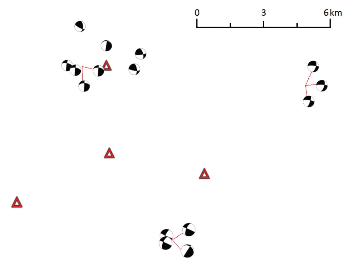
Note that the selected events group spatially into several locations corresponding to seismic swarms. The mechanisms of events from each swarm are very similar to one another, indicating that each swarm activated one fault. The mechanisms could be interpreted as mainly strike-slip on north-east oriented faults. They are also similar to the mechanism of the mainshock of the Enola intraplate swarm from May 4th, 2001 (M=4.4) located in the eastern Arkoma Basin (Rabak et al., 2010) and to the mechanism of the event from October 11th, 2010 (M=4.0) located on the Guy-Greenbrier Fault (Horton, 2012). Similar mechanisms – strike-slip with a small component of thrusting – were also determined for the 1982 Enola earthquake swarm (Chiu et al., 1984).

Stress State

As we observed a statistically significant sample of seismic events on various faults, we were able to invert for the stress field that caused these natural events. The inversion was performed using 1° angular steps for the stress orientation. The trace of the stress tensor was assumed to be zero and σ1 was set to be 1. The result of the inversion is shown in Figure 2. The optimum orientations of the principal stresses are (azimuth/plunge): σ₁ = 237°/22°, σ₂ = 13°/60° and σ₃ = 139°/19° and the optimum shape ratio is Φ = 0.822. The azimuth is measured clockwise from the north and the plunge is measured downwards from the horizontal plane.

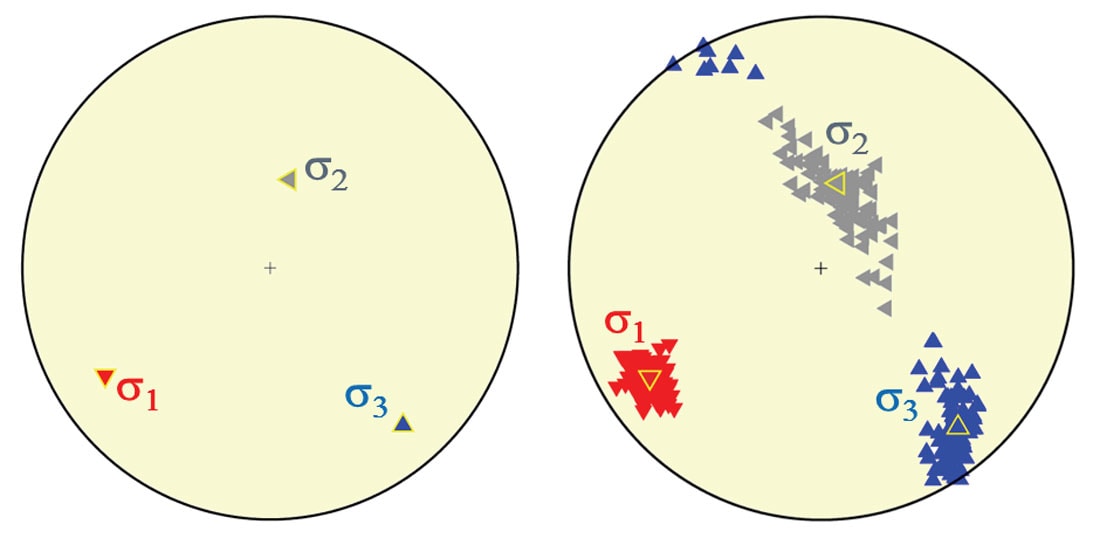
To estimate the stability and the error of our solutions, we have applied the jack-knife technique (Efron and Stein, 1981). That is, we have computed the orientations of the principal stress axes and the stress ratio from the subset of the data that had one or a few focal mechanisms removed to estimate the stability in the determination of the orientation of σ₁, σ₂ and σ₃, and the stress ratio Φ. The number of focal mechanisms varied from 15 (total set) down to 4. The test was repeated many times and the resulting orientation of σ₁, σ₂, σ₃, and stress ratio Φ were stacked. The stacked solutions may be considered as an estimate of the confidence zone. Contrary to constructing it from the probability density function, however, we cannot easily assign it the probability content. As can be seen in Figure 2, the resulting plots of the maximum stress axis, σ₁, are clustered tightly without outliers. This observation indicates a good resolution of stress orientation and the fact that the stress field is approximately homogenous in the investigated region. The minimum and medium stress axes, σ₁ and σ₂, have a larger scatter. The maximum (σ₁) and minimum (σ₃) stress axes are almost horizontal and the medium stress axis (σ₂) is almost vertical. The azimuth of the maximum horizontal stress SHmax (corresponding σ1) is 57° (237°).

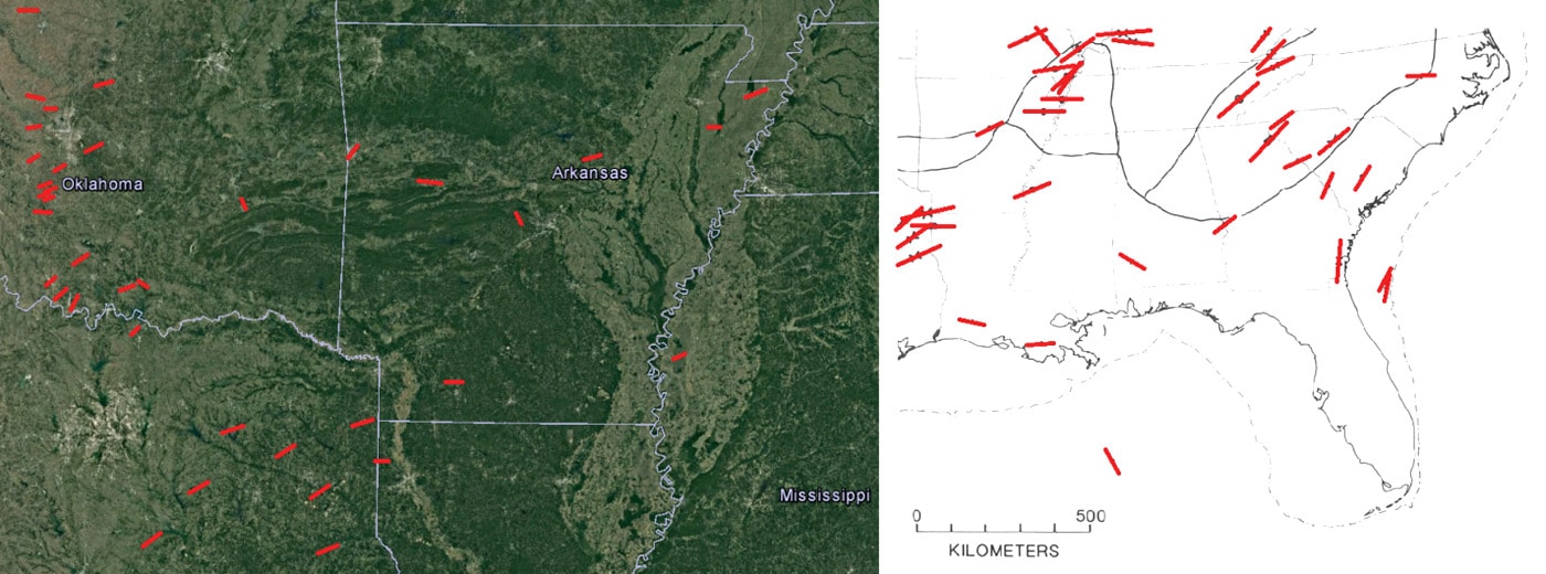
The stress state obtained from the source mechanisms of the events occurring in the study area since the new monitoring network was established is in a good agreement with the stress pattern indicated from the World Stress Map (Heidbach et al., 2008) and from the tectonic stress field of the continental U.S. (Zoback and Zoback, 1989) as shown in Figure 3. The possible fault planes are preferentially oriented in the direction of SHmax and are consistent with strike-slip motion on nearly vertical fault planes.

Conclusions

We have shown that the seismic monitoring network with only four stations is capable of characterizing the stress state at the selected site before the injection. This monitoring required approximately 15 months of operation and resulted in the mapping of active faults.