Introduction
With the increased seismicity rate in the Western Canada Sedimentary Basin (WCSB), accurate determination of local magnitude (ML) using data from regional seismograph networks is a vital task for induced seismicity monitoring and mitigation of seismic hazard. Specific mitigation strategies have been put in place by the regulators when the induced events exceed a predefined ML threshold (Kao et al., 2016, 2018). Regulations in both British Columbia and Alberta impose suspension orders to temporarily halt injection operations in case of an induced event with ML 4.0 or larger.
Currently, Natural Resources Canada (NRCan) follows the Richter (1935) scale, which was originally designed for southern California, to determine the ML of seismic events in western Canada. One key difference between the Richter’s calculation of ML and the NRCan’s is that the former measures the maximum amplitude from horizontal components, whereas the later uses the vertical component. Moreover, the original Richter method uses the largest recorded amplitude (on a Wood-Anderson, WA, seismometer) regardless of seismic phases, whereas NRCan uses the window encompassing the S phase.
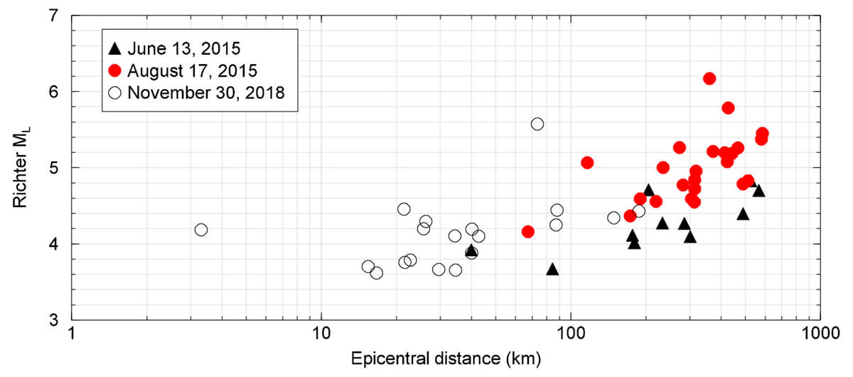
Yenier (2017; referred to hereafter as Y17) observed an increase in the ML values reported by NRCan with distance (Figure 1) and concluded that the distance correction terms in the original Richter scale may not be suitable for WCSB. Using data from horizontal components, Y17 also obtained distance correction terms to account for the attenuation effects across WCSB. In a similar study, Babaie Mahani and Kao (2019; referred to hereafter as BMK19) estimated the distance correction terms (i.e. proper adjustment to the original Richter ML table) when the vertical component is used in the calculation.
In this report, we provide an update on the distance correction terms of BMK19 using newly available data. We also provide comparisons between the result obtained by the updated model and those of Y17 and BMK19. Moreover, using the dataset from a local seismograph array established by one of the operators in the region, we analyze the performance of each model and verify their consistency in the determination of ML for induced earthquakes within WCSB.
Dataset
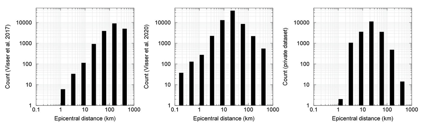
In BMK19, the analysis was done with the vertical WA amplitudes taken from the comprehensive catalogue of local and regional earthquakes in WCSB compiled by Visser et al. (2017) for the period of 2014-2016 (inclusive). The dataset includes 18918 amplitude values recorded at epicentral distances between 0.4 and 600 km from 4916 earthquakes. Taking advantage of the recent increase in the number of local and regional seismograph stations, Visser et al. (2020) provided another comprehensive dataset for the period of 2017-2018 (inclusive). The new dataset includes 63883 vertical WA amplitudes from 10693 earthquakes within the southern Montney play in northeast British Columbia recorded at epicentral distances between 0.1 and 600 km. The new dataset provides an opportunity to review the correction factors obtained by BMK19 and to improve the accuracy of these factors in light of a bigger dataset. The combined dataset (i.e. Visser et al., 2017 and 2020) includes a total of 82801 vertical WA amplitudes at epicentral distances between 0.1 and 600 km from 15609 earthquakes. The other dataset used in this study is provided by a local operator, consisting of peak amplitude measurements from a local seismograph array in west central Alberta. This dataset includes 19770 WA amplitude values (vertical and horizontal components) from 948 earthquakes. Note that the private dataset is only used for the purpose of comparison of the results. Figure 2 shows the number of data samples as a function of epicentral distance.
Methodology
Richter (1935) devised the first systematic measure of the size of an earthquake using a small dataset from southern California. The most important input parameter in the magnitude calculation is the maximum zero-to-peak amplitude measured from the horizontal components of ground displacement, regardless of the wave type, recorded on WA torsion seismometers. Since then, this method has been widely adopted around the globe with various modifications for different tectonic regions (e.g. Hutton and Boore, 1987; Savage and Anderson, 1995; Uhrhammer et al., 2011; Ottemoller and Sargeant, 2013). To preserve the original sensor type, WA amplitudes are synthetically obtained through deconvolution of the recording sensor’s instrument response (non-WA sensors) from the recorded waveform and convolution with the WA type instrument response.
The Richter magnitude scale is defined as

where A is the recorded amplitude, in mm, on a WA seismometer, A0 is the distance correction term for the recorded amplitude, and S is a correction term for each station that accounts for any systematic amplitude difference such as local site effect. Richter (1935) determined the S terms for each station by taking the average of the magnitude differences between the values obtained for individual stations and the mean value for the event. A0 at each distance was obtained by defining the zero magnitude (ignoring the S term) at a distance of 100 km (A = 0.001 mm). Here, we obtain A0 for WCSB through regression of the WA amplitudes, as compiled by Visser et al. (2017, 2020), against a given model that accounts for the attenuation of ground motion amplitudes in the WCSB.
The model for the distance correction can be defined as (Rezapour and Rezaei, 2011)

where Rhypo is hypocentral distance, and n and k are the corrections for geometrical spreading and anelastic attenuation, respectively. Equation (2) is written in such a way that for the reference distance of 100 km, the corresponding amplitude is 0.001 mm (-log(A0) = 3) to maintain the consistency with the original definition of ML.
Equations (1) and (2) can be combined and re-arranged to give

where ε is the residuals in log units. We obtain n, k, ML, and S by constructing the linear inverse equation of d = Gm (Menke, 1984) where d is observed data (log(A) + 3.0) and m is the model parameter vector (n, k, ML, and S) to be determined. G is the kernel matrix, which relates d to m. In solving for the model parameters, the correction term for each station (S) is obtained simultaneously. Here, the correction terms for stations are computed relative to the average site condition by constraining the S terms to attain zero when averaged over all stations.
In modeling the attenuation, an important factor is the shape or functional form of geometrical spreading, which is characterized by n. Linear, bi-linear, and tri-linear functional forms have been used to model the attenuation of ground motion from geometrical spreading (e.g. Babaie Mahani and Atkinson, 2012). Following BMK19, we use a bi-linear function with the transition distance at 85 km as
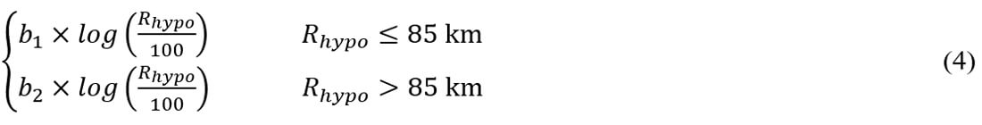
to model the effect of geometrical spreading (n), where b1 and b2 are the coefficients to be determined.
In theory, the ML value obtained from the horizontal component of ground motions should be consistent with that from the vertical component, as long as the correction terms are properly calibrated. Historically NRCan chose to use the vertical-component peak amplitude in the ML calculation for two reasons. First, single-component (vertical), short-period sensors were installed in many seismograph stations of the Canadian National Seismograph Network (CNSN). Therefore, using vertical-component data would maximize the number of available stations in the calculation, which is especially important for regions with very sparse station coverage. We note, however, that all CNSN stations are now equipped with 3-component broadband sensors. The second reason is that the level of background noise on the vertical component is generally lower than that on the horizontal components. To maximize our data resolution, we follow NRCan’s convention of using vertical-component measurements in BMK19 and this study.
Results
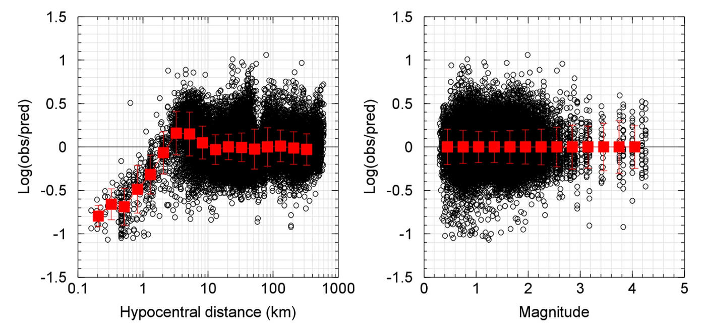
Using Equations (3) and (4), model parameters b1, b2, k, ML, and S are obtained through the least-square inversion in MATLAB. Here, we only use events with at least 8 observations and stations that recorded at least 8 events (3575 events with 33994 vertical WA amplitudes at 56 stations). Figure 3 shows the results of regression by plotting the residuals versus hypocentral distance and magnitude. There is a clear over-prediction at hypocentral distances < 2 km. Although the epicentral distance of the recorded events can be as low as 0.1 km, the focal depths of most events are more than 2 km. Therefore, samples with hypocentral distances < 2 km may correspond to very shallow events in the earthquake catalogues or mislocated events due to insufficient data constraint. For this reason, the validity of our model would be for hypocentral distances of > 2 km. Beyond 2 km there are no trends in the residuals with distance. Similar results can be seen for the relationship between residual and magnitude, as no trend can be recognized across the entire magnitude range. The lack of an apparent trend means that the inversion was successful assuming the functional forms for the attenuation and geometric spreading.
Our updated distance correction term, -log(A0), for WCSB is
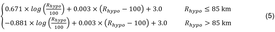
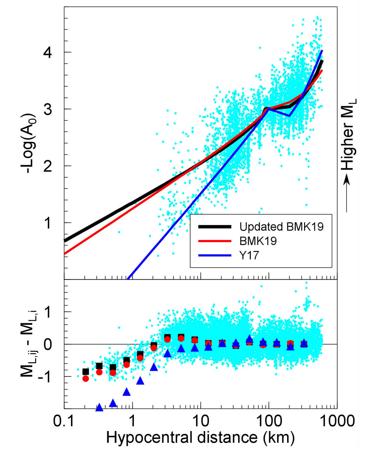
Figure 4 (top panel) shows the comparison of the -log(A0) term from Y17, BMK19, and the updated model with respect to hypocentral distance. All data samples are normalized by the average amplitude in the distance bin of 90-110 km such that the distance correction term is 3 at 100 km. The three models are similar for distances around 100 km and above. At closer distances, the updated model shows small improvement compared to BMK19, whereas Y17 gives significantly smaller values for -log(A0) (and therefore smaller ML). This can also be seen in Figure 4 (bottom panel) which shows, for each event i, the difference between the ML value derived from the peak amplitude at each station j (ML,ij) and the event’s final ML value (ML,i, defined as the median of all ML,ij). The observed under-prediction by Y17 at hypocentral distances < 10 km is mainly due to the difference between vertical and horizontal amplitudes. As mentioned before, whilst Y17 use the horizontal amplitudes in the ML calculation, BMK19 and the updated model in this study both use the vertical component of ground motion. The lower amplitudes of shear waves on the horizontal components compared to the vertical component at short distances can explain the discrepancy between the models. In Table 1, the correction term for each station (S) is compiled.
The Private Dataset
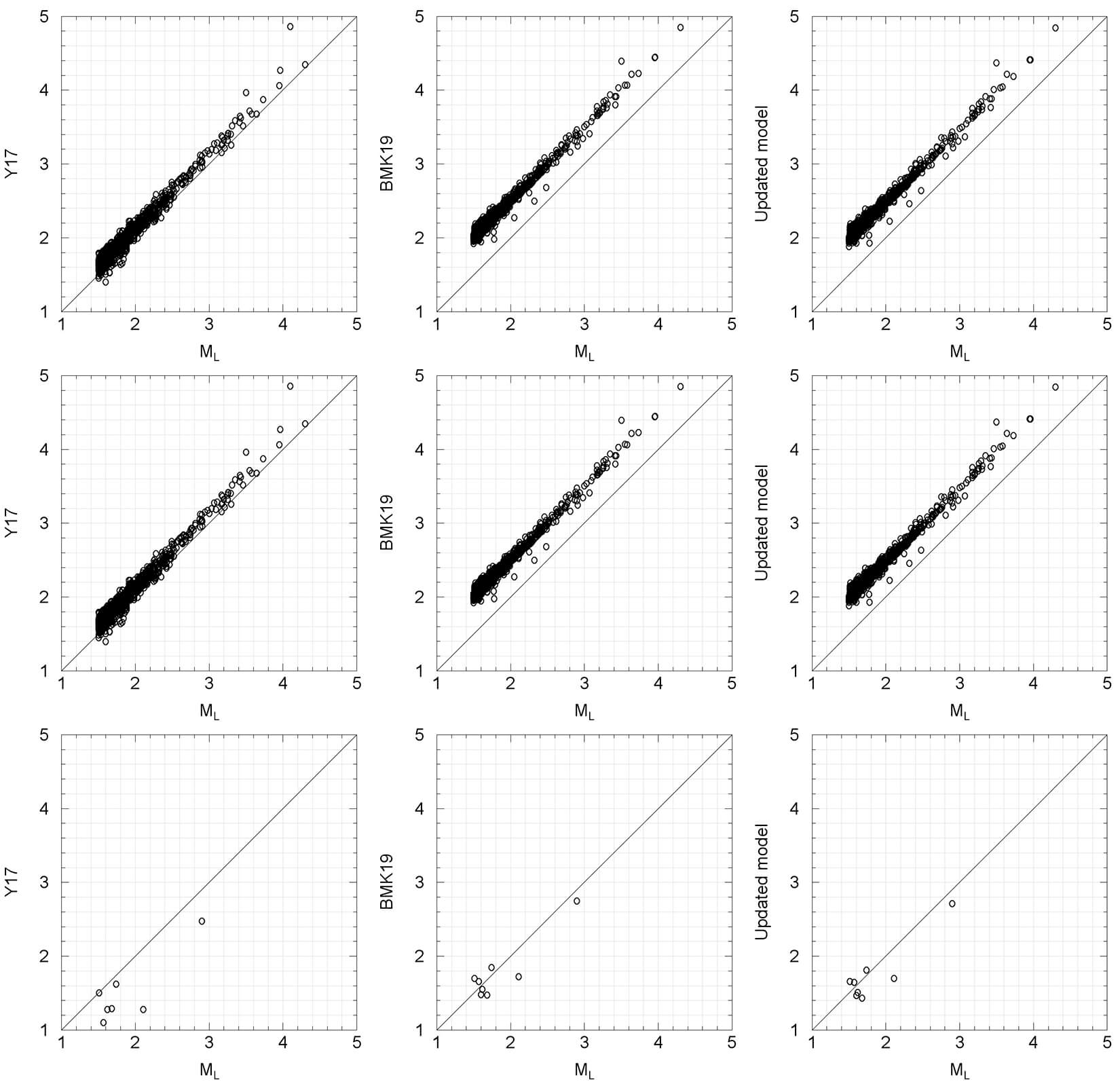
Figure 5 shows the comparison between ML values as reported in the private dataset and those obtained using Y17, BMK19, and the updated model. In the top row, we use all of the available WA amplitudes, including both vertical and horizontal amplitudes, whereas in the middle and bottom rows, only the horizontal and vertical components are used, respectively. It is clear in Figure 5 that, for the top and middle row, ML values obtained by Y17 match the reported values in the private dataset very well, while BMK19 and the updated model over-estimate for all magnitudes. On the other hand, BMK19 and the updated model match the values reported in the private dataset very well when the ML calculation is based on measurements from the vertical component despite the small number of available samples. As expected, Y17 under-predicts the ML value for all magnitudes in this case.
| Station | Latitude | Longitude | S |
|---|---|---|---|
| Table 1. Correction term (S in Equation 1) for each seismograph station. | |||
| ATHA | 54.7137 | -113.31 | -0.0484 |
| BDMTA | 54.8129 | -118.91 | 0.1263 |
| BLBC | 52.0434 | -119.24 | 0.2178 |
| BMBC | 56.0449 | -122.13 | 0.0542 |
| BRLDA | 54.092 | -117.4 | -0.0331 |
| DEDWA | 56.6446 | -117.39 | 0.0643 |
| DLBC | 58.4372 | -130.03 | 0.2261 |
| EDM | 53.2217 | -113.35 | 0.2105 |
| EGLEA | 54.4571 | -116.44 | -0.0357 |
| FAIRA | 56.1087 | -118.86 | 0.0064 |
| FNBB | 58.8903 | -123.01 | 0.1137 |
| FSB | 54.4767 | -124.33 | 0.3241 |
| FSJB | 54.4588 | -124.29 | 0.2315 |
| GODA | 55.8392 | -119.57 | -0.7906 |
| HILA | 58.5561 | -117.02 | -1.198 |
| KIMIA | 55.9938 | -116.61 | 0.0475 |
| KITB | 54.0779 | -128.64 | 0.1576 |
| LGPLA | 53.1165 | -115.36 | 0.1159 |
| LLLB | 50.609 | -121.88 | 0.2491 |
| MANA | 56.8554 | -117.64 | -0.003 |
| MG01 | 56.0548 | -120.64 | -0.3797 |
| MG02 | 55.8668 | -120.08 | -0.0996 |
| MG03 | 55.9122 | -120.44 | -0.0518 |
| MG04 | 55.9914 | -120.34 | -0.1007 |
| MG05 | 55.8951 | -120.3 | -0.0594 |
| MG06 | 55.8721 | -120.04 | -0.1393 |
| MG07 | 55.7836 | -120.4 | 0.0819 |
| MG08 | 55.8412 | -120.87 | 0.0085 |
| MG09 | 55.7442 | -120.78 | 0.0246 |
| MNB | 52.1983 | -118.38 | 0.2141 |
| MONT1 | 55.9102 | -120.59 | 0.0485 |
| MONT2 | 56.0197 | -120.05 | -0.0274 |
| MONT3 | 56.0058 | -120.45 | 0.1339 |
| MONT4 | 57.3184 | -122.71 | -0.1954 |
| MONT5 | 57.0269 | -122.34 | -0.0921 |
| MONT6 | 56.1103 | -121.02 | -0.2419 |
| NAB1 | 56.7663 | -121.26 | 0.1325 |
| NAB2 | 58.595 | -119.17 | -0.0295 |
| NBC1 | 59.6559 | -123.82 | -0.0204 |
| NBC2 | 59.7735 | -122.49 | 0.0231 |
| NBC3 | 59.6372 | -120.67 | 0.1948 |
| NBC4 | 55.6873 | -120.66 | 0.1518 |
| NBC5 | 57.5231 | -122.68 | 0.1046 |
| NBC6 | 58.5839 | -121.33 | 0.0445 |
| NBC7 | 56.2678 | -120.84 | -0.233 |
| NBC8 | 56.5731 | -122.4 | 0.115 |
| RDEA | 56.5513 | -115.32 | -0.1899 |
| SNUFA | 54.6781 | -117.54 | -0.0296 |
| STPRA | 55.6606 | -115.83 | -0.0001 |
| SWHSA | 54.8994 | -116.75 | 0.0963 |
| TD002 | 53.4394 | -114.39 | 0.0615 |
| TD009 | 52.3206 | -116.32 | -0.054 |
| TONYA | 54.4054 | -117.49 | 0.1052 |
| UBRB | 52.8918 | -124.08 | 0.1818 |
| WAPA | 55.1833 | -119.25 | 0.1325 |
| WTMTA | 55.6942 | -119.24 | 0.0522 |
Conclusion
Using a comprehensive earthquake dataset for the period of 2014-2018 (inclusive), we provide an update on the distance correction term in the ML calculation of local earthquakes in WCSB. A total of 33994 vertical Wood-Anderson amplitudes from 3575 earthquakes recorded at 56 local and regional seismograph stations are used in the regression. Our revised formula can better characterize the attenuation effect associated with the unique geological and tectonic configuration of WCSB. As a result, it provides higher consistency between ML values calculated at individual stations and the final event ML over a wide hypocentral distance range from 2 to 600 km, and therefore is a reasonable alternative to the original Richter formula for regulatory purposes in northeastern BC and western Alberta.

Acknowledgements
Waveform data used in this study are obtained from the Canadian Hazard Information Service and the Data Management Center of the Incorporated Research Institutions for Seismology (IRIS). The private dataset is provided to NRCan under a data sharing agreement. This research is partially supported by NRCan’s Energy Innovation Program, Geological Survey of Canada Environmental Geoscience Program, and a research grant from Geoscience BC. NRCan contribution 20200022.


Join the Conversation
Interested in starting, or contributing to a conversation about an article or issue of the RECORDER? Join our CSEG LinkedIn Group.
Share This Article