Summary
Identifying subtle faults at or below the limits of seismic resolution and predicting fractures associated with folds and flexures is one of the major objectives of careful seismic interpretation. With the common use of 3D seismic in the late 1980s, 1st derivative based horizon dip magnitude and dip azimuth were found to enhance faults that were otherwise difficult to see. More recently, 2nd derivative based curvature maps have carried this process a step further. Horizon-based curvature computation has become available in the commercial workstation environment, putting these tools in the hands of geoscientists who do not have access to processing software and do not have time or inclination to program. While more interpretationally intensive, horizon-based curvature workflows can be modified such that they can approximate some of the more important aspects of volumetric estimates of curvature, including improved accuracy and estimation of long wavelength curvature. Equally important, workstation scaling and display workflows need to be modified in order to reflect the dual polarity nature of most of the curvature measures.
Introduction
Seismic interpreters have used attribute maps for fault interpretation since the introduction of 3D seismic data. Rijks and Jaufred (1991) showed that dip magnitude and dip azimuth can illuminate subtle faults having a displacement significantly less than the size of a seismic wavelet. Coherence (Bahorich and Farmer, 1995) and Sobel-filter-based edge detectors (Luo et al., 1996) measured lateral changes in seismic waveforms and amplitude. More recently, curvature attributes have been found to be useful in delineating faults and predicting fracture orientation and distribution (Roberts, 2001, Hakami et al, 2004). There are different curvature measures that can be used, each having its own characteristic property. Lisle (1994) discussed the correlation of Gaussian curvature to open fractures measured on an outcrop. Hart (2002) showed that strike curvature is highly correlated to open fractures in NW New Mexico. In contrast, Stevenson (2006) found that the dip component of curvature is correlated to open fractures in the Austin Chalk formation of Central Texas. Ericsson et al. (1988) demonstrated the relationship between production and curvature. While direct prediction of open fractures using curvature requires a significant amount of calibration through the use of production, tracer, image log, or microseismic measurements, curvature images also serve as a powerful aid to conventional structural and stratigraphic interpretation. Curvature is particularly useful in mapping faults that are smeared due to inaccurate migration. Sigismondi and Soldo (2003) have used larger analysis windows thereby computing maximum curvature at different scales to extract subtle features that are much less obvious from the original time/structure map. Bergbauer et al. (2003) also compute curvature at different wavelengths by filtering the input horizon picks in kx- ky space. Al-Dossary and Marfurt (2006) extend this latter concept to volumetric estimates of curvature by replacing the kx-ky filter with a more tractable x-y convolutional operator.
While volumetric curvature has several significant advances over horizon-based curvature, not least of which is circumventing the need to pick regions through which no continuous surface exists, we understand that most interpreters do not have access to such processing software and compute engines. In this paper, we therefore attempt to discuss how to use convenient filtering and display techniques available on modern interpretation software to generate horizon-based curvature estimates of similar quality to horizon slices through volumetric estimates.
We illustrate these workflows and discuss their usefulness in terms of their applications to two 3D seismic volumes, one from Alberta and the other from British Columbia, Canada.
Definition and types of curvature
Curvature can be defined as the reciprocal of the radius of a circle that is tangent to the given curve at a point. Thus curvature will be large for a curve that is bent more and will be zero for a straight line. Mathematically, curvature may simply be defined as a second order derivative of the curve. If the radii of the circles at the point of contact on the curve are replaced by normal vectors, it is possible to assign a sign to curvature for different shapes, as was proposed by Roberts (2001). Diverging vectors on the curve are associated with anticlines , converging vectors with synclines and parallel vectors with planar surfaces (which have zero curvature). The concept of curvature can be conveniently extended to three dimensional surfaces by considering such a surface being intersected by a plane and describing a curve. Curvature can then be calculated at any point on this curve. If a given surface is cut by planes that are orthogonal to it, the curvature measures are referred to as normal curvatures (Roberts 2001). Of the family of curves that are formed this way, there exist just two curves perpendicular to each other, where one represents the maximum and the other the minimum curvature. Both these attributes, with their sign and magnitude, are useful, as faults can be clearly seen on such displays.
Curvature computation in practice
For most interpreters operating on a workstation, curvature is usually computed by fitting a quadratic surface z(x, y) of the form

to an interpreted horizon using least-squares or some other approximation method. This yields the coefficients given in equation 1 from which other curvature measures can be derived, such as minimum and maximum curvatures, principal curvatures, most-positive, most-negative, dip curvature, strike curvature, curvedness and shape index. Since curvature is a second derivative of the picked surface, its application to interpreted horizons needs to be done carefully in that it tends to exacerbate the finer detail and the noise as well. Horizons picked on noisy surface seismic data or data contaminated with mis-picks could lead to misleading curvature measures. Consequently, it is advisable to run spatial filtering on horizon surfaces, taking care to remove noise while retaining geologic detail. Most commercial software provides a basic suite of spatial filters that could be used for the purpose including mean, median, directional derivative, and sharpening:
1) The mean filter removes random noise and computes the mean or average of the values that fall within the chosen aperture. The mean filter applied to an interpreted surface enhances long wavelength and suppresses short wavelength curvature components. Iterative application of a mean filter to a map (i.e. applying the filter successively) will enhance longer and longer wavelength features. Conversely, if we subtract this long-wavelength map from the original broadband wavelength map and then compute curvature on the residual, we obtain curvature images that enhance short wavelength features.
2) The median filter also removes random noise but preserves edges, which in the case of a picked horizon will include discrete offsets, such as encountered at a fault. The median filter can also be applied iteratively, which will reduce random noise at each iteration, but will not significantly increase the high frequency geologic component of the surface.
3) Derivative (sometimes call Sobel) filters increase the high frequency content off the data, and are commonly computed using a 3 x 3 mask oriented in a particular direction as shown below:

Since curvature is a 2nd derivative operation applied to an interpreted surface, adding an additional derivative only further exacerbates any noise problems.
4) The sharpening (also call Laplacian) filter computes the 2nd derivative of the inline and crossline components of dip and adds the results. Inspection of formula provided by Roberts will show that the sharpening filter is closely related to the mean curvature, discussed below.
(Data courtesy: Arcis Corporation, Calgary).
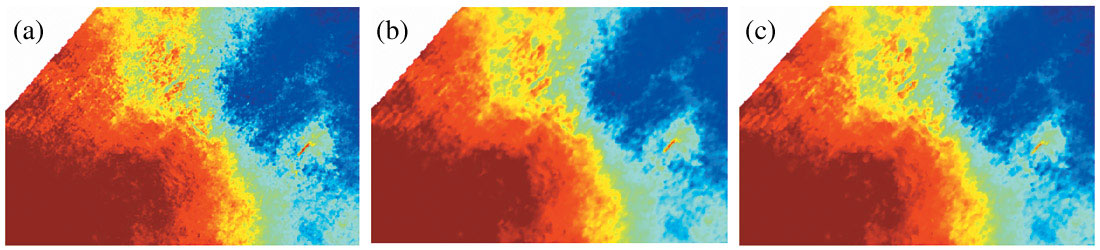
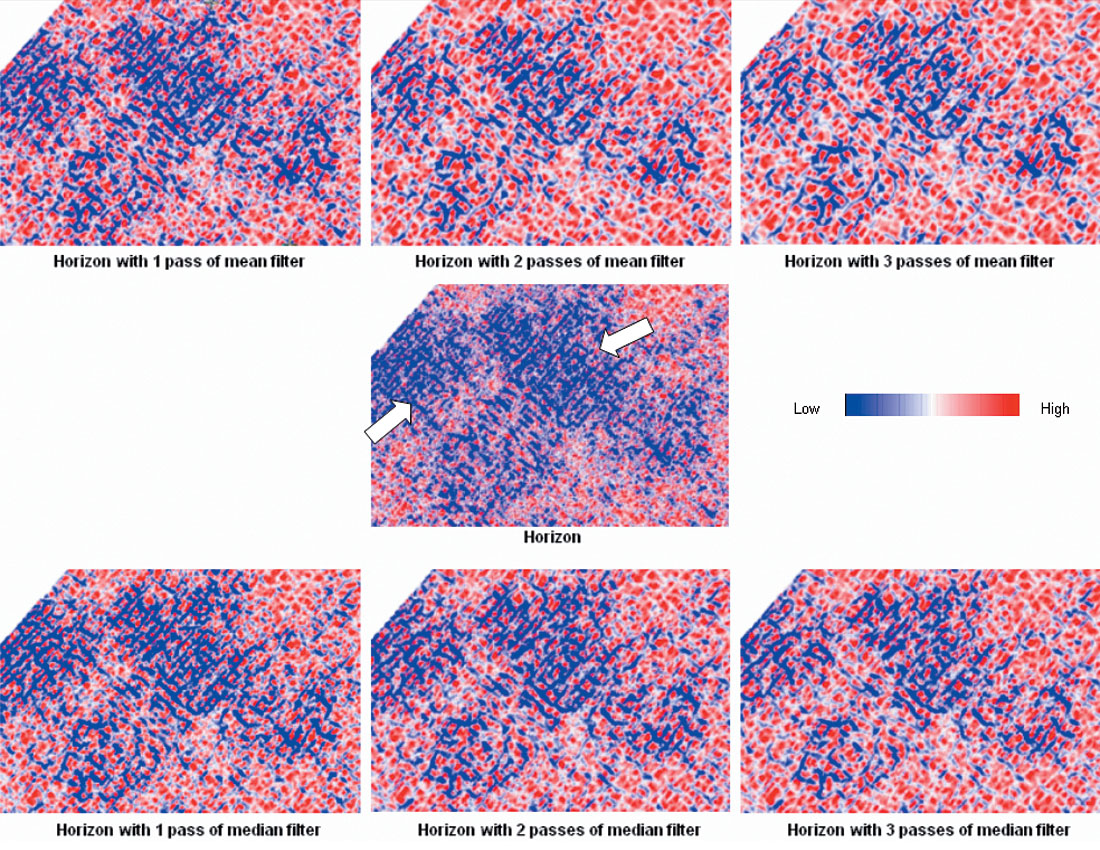
To illustrate these filters, we manually picked a horizon surface (shown in Figure 1a), line by line, representing a limestone marker from a 3D volume from south central Alberta, ensuring there were no mis-picks on the surface. We then computed most-negative curvature of this surface without filtering and display the result in the center panel of Figure 2. Note patches showing a discrete mesh of faults (white arrow). This horizon was successively passed through a 3x3 mean filter (shown in Figure 1b) and the most-negative curvature generated in each pass. As seen in the upper panel of Figure 2, with each successive pass of the mean filter the background jitter is reduced and the focusing of the events increases. The same process was repeated with a 3x3 median filter (shown in Figure 1c), where we display the corresponding images in the lower panel of Figure 2. As expected, the median filter smooths random oscillations but preserves the major edges in the horizon time/structure map, resulting in crisper most-negative curvature displays.
(Data courtesy: Arcis Corporation, Calgary).
Picking the horizon for accurate curvature computation
In a recent presentation, Blumentritt (2006) found that the quality of volumetric estimates of curvature (that precomputed dip and azimuth volumes using a finite vertical analysis window of say, +/- 10 ms) could be approached better by picking the zero crossing. He explains this improvement in that noise added to the flat part of a peak or trough can significantly move the autopick. The same noise added to the much steeper zero crossing has a much smaller effect. Following Blumentritt (2006) we then recommend the following workflow:
- Pick the data peak or trough as fits your well tie,
- Compute the quadrature of the seismic data,
- Snap the original picks to the zero crossing,
- Compute the curvature from these snapped picks to the zero crossings.
If the data at the peak or trough is nearly flat, moving it slightly will not significantly impact the amplitude extractions.
Curvature attributes
Example 1
(Data courtesy: Arcis Corporation, Calgary).
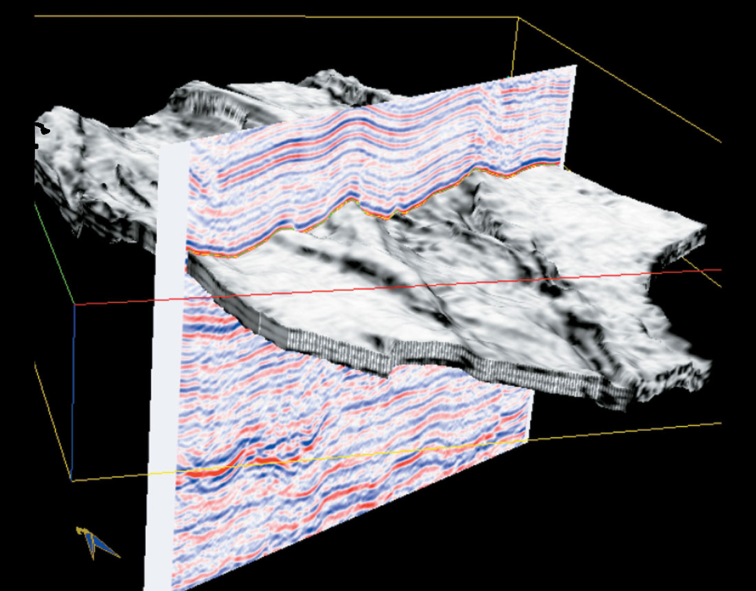
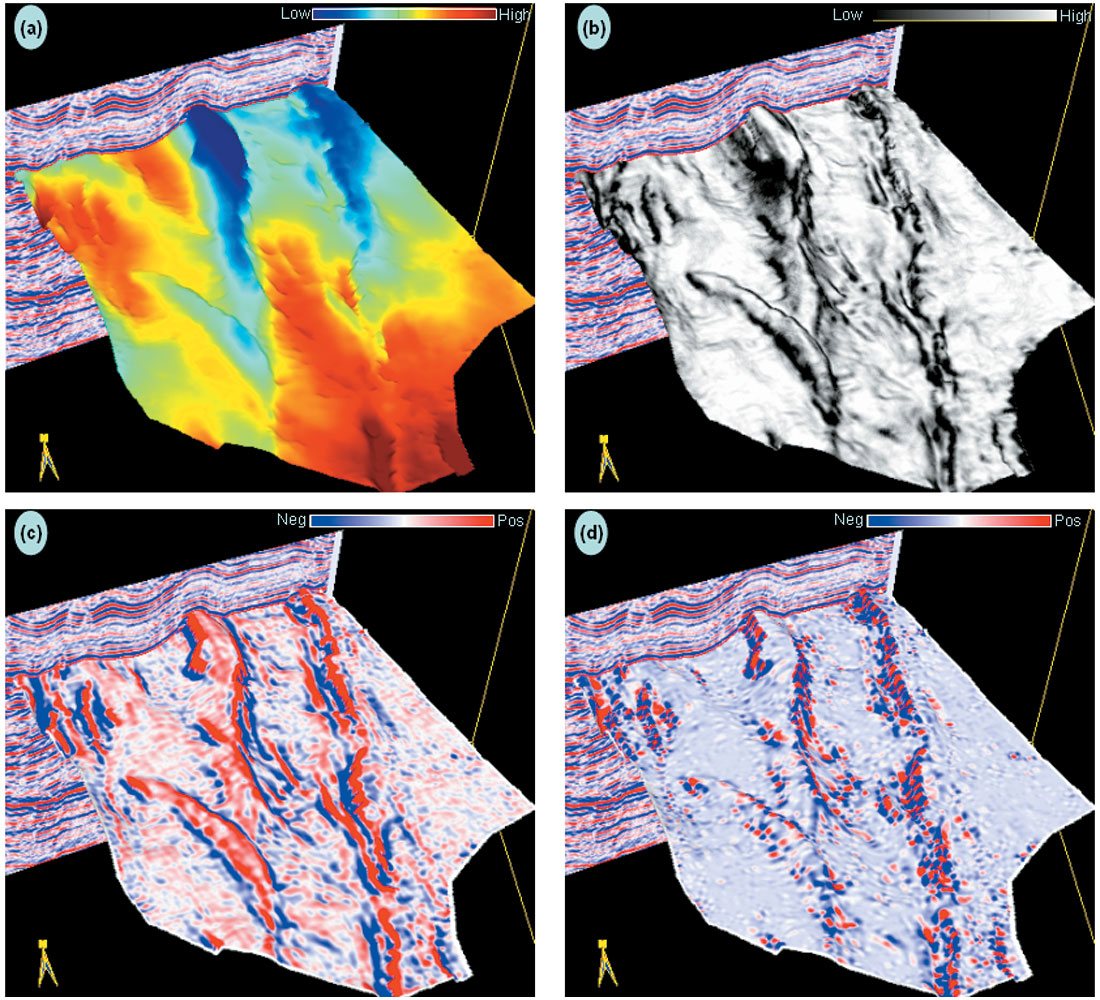
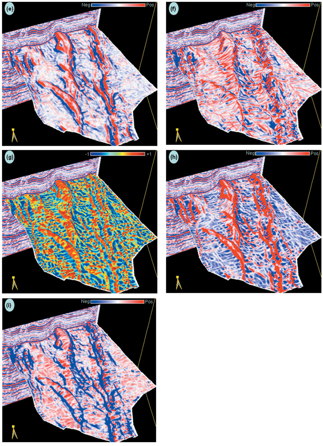
Figure 3 shows a coherence strat-cube being intersected by a seismic line from a 3D seismic volume from central-north British Columbia, Canada. [A strat-cube is a sub-volume of seismic data or attributes that are either parallel to a picked horizon (commonly called a flattened subvolume) or interpolated at equal time increments between two non-parallel picked horizons]. A number of faults can be seen on the vertical seismic section. The top of the coherence strat-cube was chosen to be the base of the Belloy formation (shown in Figure 4a). We illustrate the basic curvature attributes along the picked Belloy surface in Figures 4c-f:
(Data courtesy: Arcis Corporation, Calgary).
Mean curvature: is defined as the average of the minimum and maximum curvature and usually dominated by maximum curvature. Visually, it may not convey any additional information, but is useful as other attributes are derived from it. Compared with coherence display (Figure 4b), the sign of mean curvature indicates the high and low shapes (Figure 4c), giving a feel for the throw of the faults. Many workers like the fact that they can estimate fault throw by the change in color pattern (e.g. Sigismundi and Soldo).
Gaussian curvature: is defined as the product of the minimum and maximum curvatures and gives a measure of distortion of a surface. While this measure has been shown to be correlated to fractures (Lisle, 1994), it does not show discrete faults either in this example (Figure 4d) or in the example presented by Roberts (2001).
Dip curvature: is the curvature extracted along the direction of dip at each analysis point and measures the rate of change of dip in the maximum dip direction. As seen in Figure 4e, dip curvature shows the throw as well as the direction of the faults clearly. Stevenson (2006) finds that dip curvature is correlated to open fractures in extensional terrains.
Strike curvature: is the curvature extracted along a direction perpendicular to the dip curvature, i.e. along strike at each analysis point. In Figure 4f, notice how on both sides of the main faults strike curvature indicates patterns connecting high with lows. In a compressional terrain, Hart et al. (2002) predict that large values of strike curvature will be correlated to open, vs. closed fractures. In a tensional terrain such as the Austin Chalk (Schnerk and Madeen, 2000), others find that dip curvature correlates with open fractures (Stevenson, 2006).
Shape index: indicates the local shape of a surface with blue indicating a bowl, cyan a valley, green a saddle, yellow a ridge, and red a dome (Figure 4g). This attribute is scale independent, such that gentle domes will be displayed the same as strong domes.
Most-positive curvature: defines the curvature that has the greatest positive value and will show anticlinal and domal features. However, negative values of the most positive curvature indicate a bowl feature (Figure 4h).
Most-negative curvature: defines the curvature that has the greatest negative value and will in general highlight synclinal and bowl features. However, positive values of the most-negative curvature indicate a dome feature (Figure 4i).
Example 2
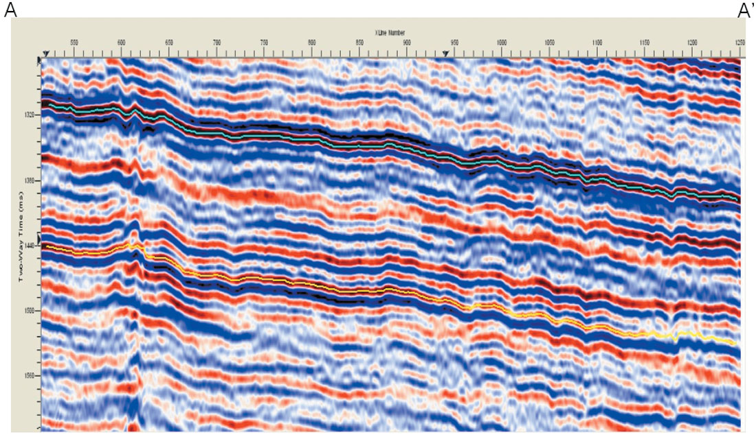
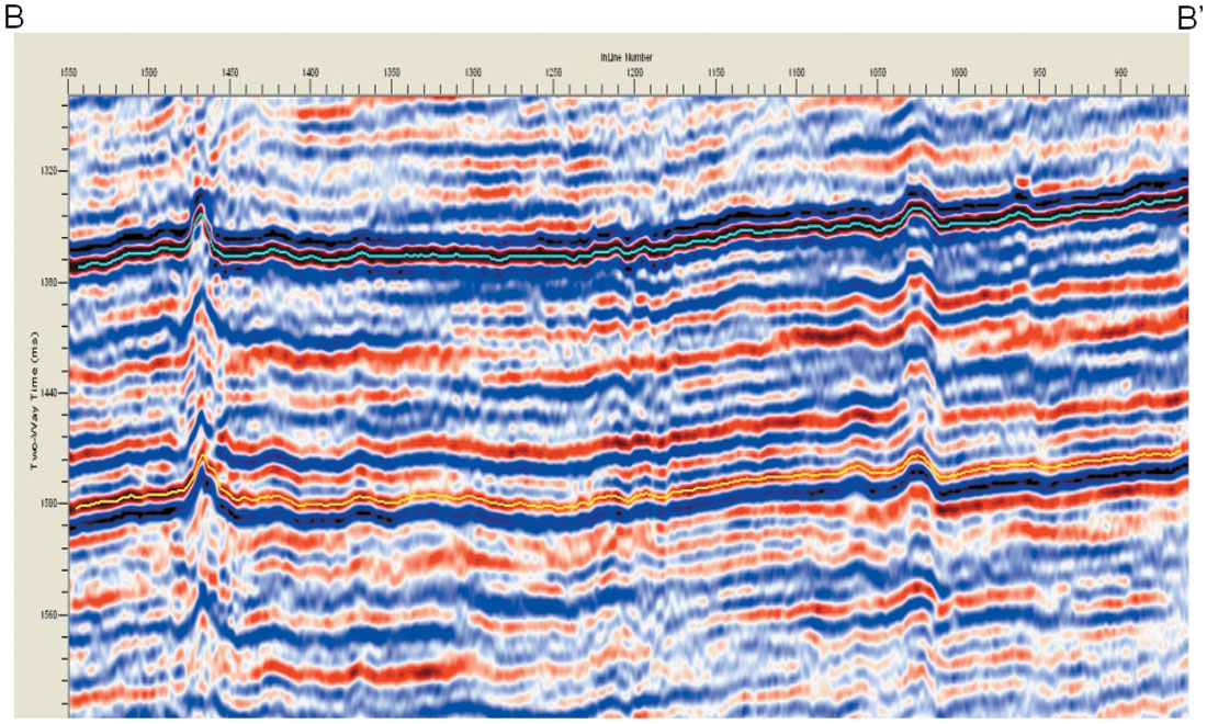
Figure 5a shows an inline and a crossline from a 3D seismic volume acquired in north-west Alberta for which we have picked two horizons and generated horizon-based curvature attributes. The upper time surface corresponding to the cyan horizon shown in Figure 5 is shown in Figure 6a and indicates two prominent fault trends, one to the top trending northeast-southwest (grey arrows) and the other to the left trending northwest- southeast direction (yellow arrows). Figure 6a also indicates the positions of the two profiles shown in Figure 5.
(Data courtesy: Arcis Corporation, Calgary).
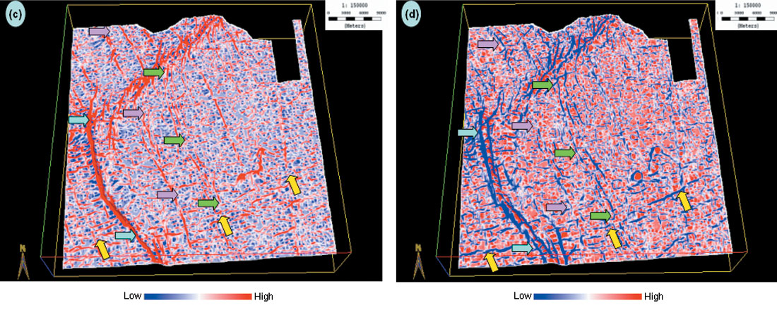
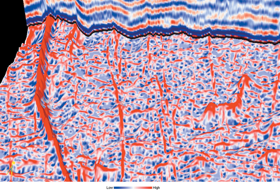
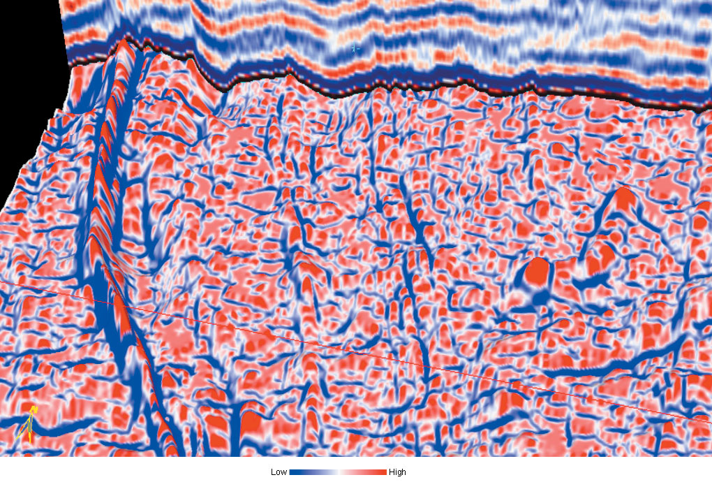
While there are hints of other faults, they do not appear so clearly. The corresponding horizon slice through the coherence volume (Figure 6b) shows up the faults much better. However, the most-positive and most-negative displays computed from the picked horizon (Figure 6c and d) show the enhanced definition of the main fault trends with greater focus and clarity. Notice, the finer definition of the faults indicated with yellow arrows and also the detail and density of the other features marked with cyan, pink and green arrows. In Figure 7a we show a zoom of the most-positive curvature horizon slice seen intersected with a seismic crossline. Notice how the red peak on the fault trend (to the left running almost north-south) correlates with the upthrown signature on the seismic. Similarly, a zoom of the most-negative curvature horizon slice intersected with an inline (Figure 7b) shows the downthrown edges on both sides of the faults highlighted in blue. Other similar features tend to stand out on the horizon slice.
(Data courtesy: Arcis Corporation, Calgary).
(Data courtesy: Arcis Corporation, Calgary).
(Data courtesy: Arcis Corporation, Calgary).
Example 3
Besides faults/fractures, other stratigraphic features also appear to be well-defined on curvature displays. In Figure 8a, we show a time surface from a 3D seismic survey from Alberta, depicting a meandering channel which is the most prominent feature that can be noticed on the display. The equivalent coherence display (Figure 8b) shows a crisper definition for the channel in addition to other features, such as the lineament is indicated with yellow arrows. The equivalent most-positive curvature display (Figure 8c) shows the linear feature more focused and clear. Cyan arrow indicates the well-defined lower leg of the channel on the curvature displays, which is not seen clearly on the coherence display. The edges of the meandering channel are well-defined on the most-positive curvature display while the thalweg of the channel can be followed clearly on the most-negative display (Figure 8d). It is important to couple the appearance of structural and stratigraphic features to a geologic model. In Alberta, some of the rocks are sufficiently old (Paleozoic to deeper Mesozoic) to have undergone differential compaction. Curvature is also successful in imaging subtle Mesozoic channels in the North Sea that have also undergone differential compaction (Helmore et al, 2004). In contrast, curvature rarely indicates channels in younger Tertiary sediments in surveys acquired in the Gulf of Mexico, where the rocks have not had time to undergo sufficient differential compaction.
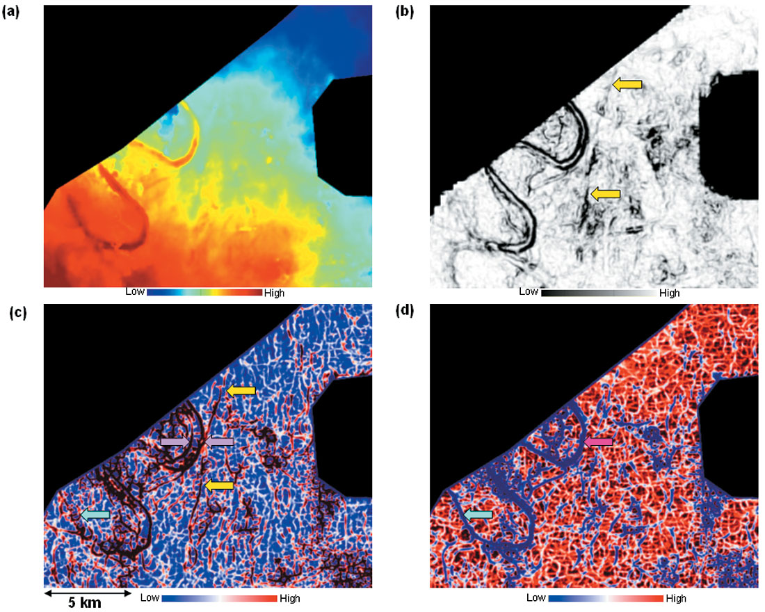
(Data courtesy: Arcis Corporation, Calgary).
Volume computation of curvature
Volume computation of curvature produces multi-spectral estimates of reflector curvature (Al Dossary and Marfurt, 2006). The method consists of choosing a moving sub-volume of data to compute curvature at every point in the 3D seismic volume. As the first step, spurious events are minimized within the subvolume and dip components are computed. Next, fractional derivatives are computed within the sub-volume to investigate multiple wavelengths of curvature – short wavelengths corresponding to intense, but highly localized fracture systems, and longer wavelengths to a wider and even distribution of fractures. Short wavelength estimates of curvature could incorporate dip information of 9 to 25 traces, while the long wavelength estimates of curvature could use dip information of 400 or more traces. Fractional derivatives are thus applied along each time slice with dip components previously estimated at each seismic bin to yield estimates of curvature.
Volume curvature estimates eliminate interpretation problems and allow us to extract curvature measures along horizons, thereby helping us understand the subsurface features better.
Example 1
Figure 9a shows the strat-slice from the most-positive curvature volume 30 ms below the horizon displayed in Figure 4. The horizon at this level is not easy to track and so the attribute volume helps in studying the fault patterns at this level. Similarly, the equivalent strat-slice extracted from the mostnegative curvature volume is shown in Figure 9b. Notice, the fault pattern is somewhat different at this level and these patterns can be studied carefully in the zone of interest.
(Data courtesy: Arcis Corporation, Calgary).
(Data courtesy: Arcis Corporation, Calgary).
Example 2
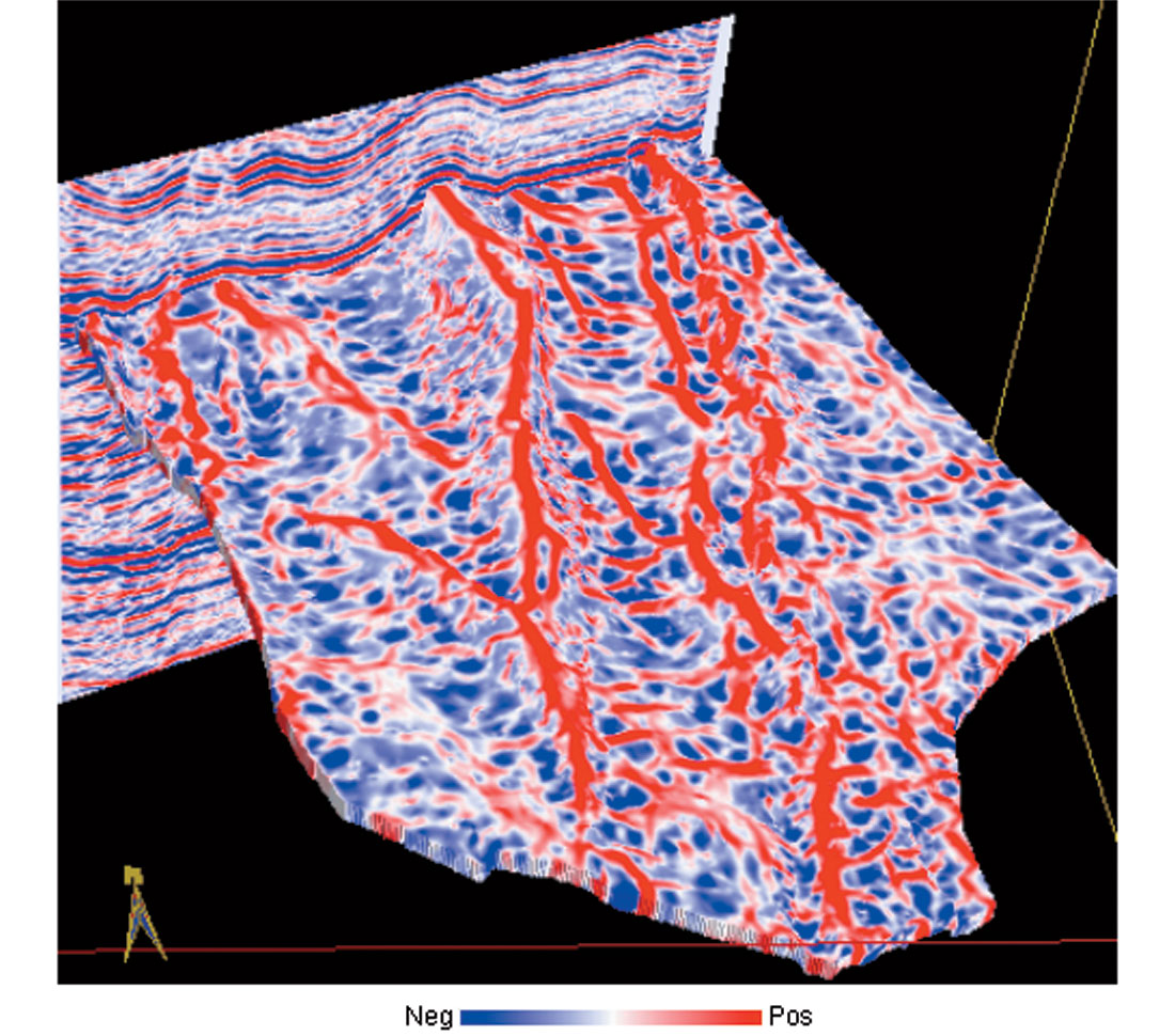
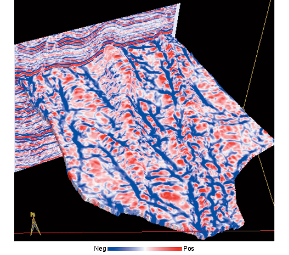
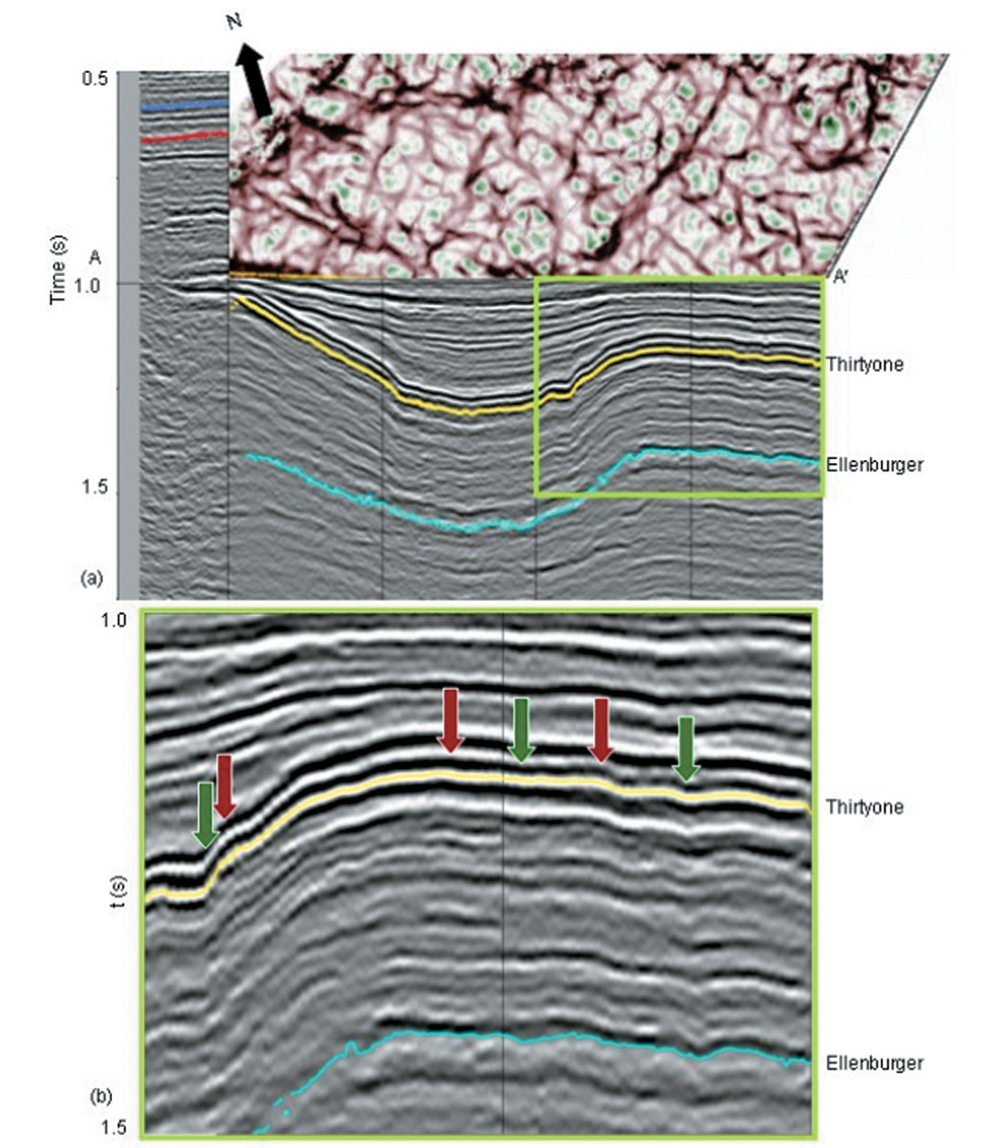
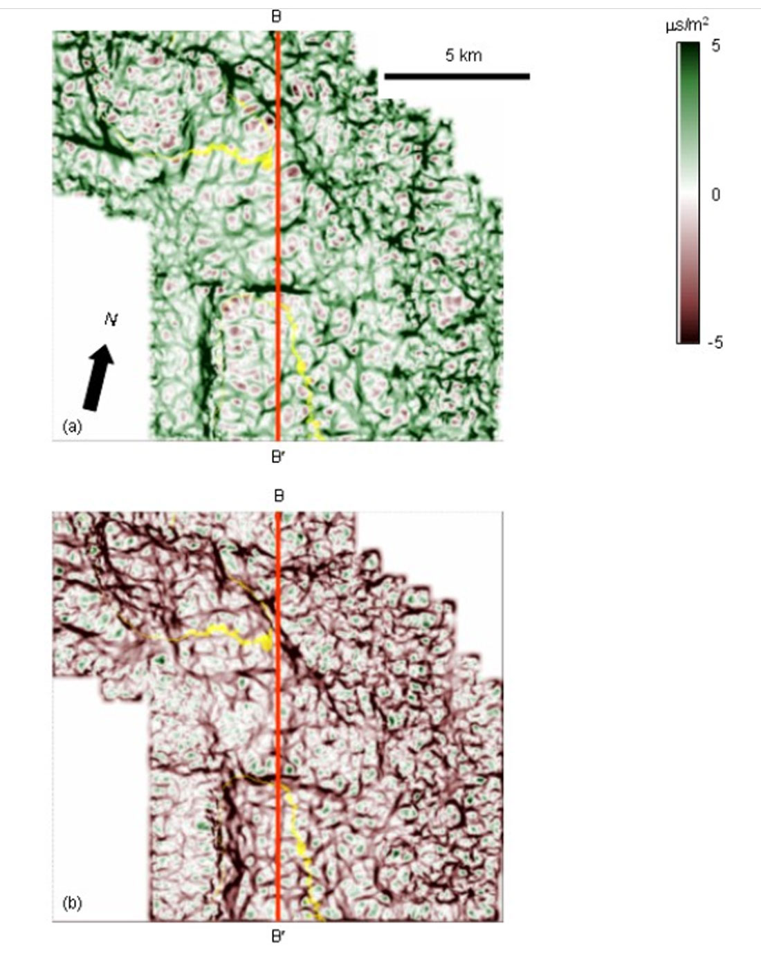
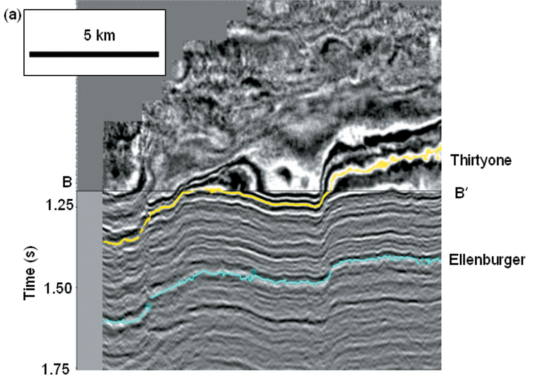
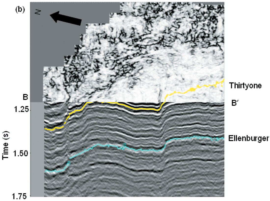
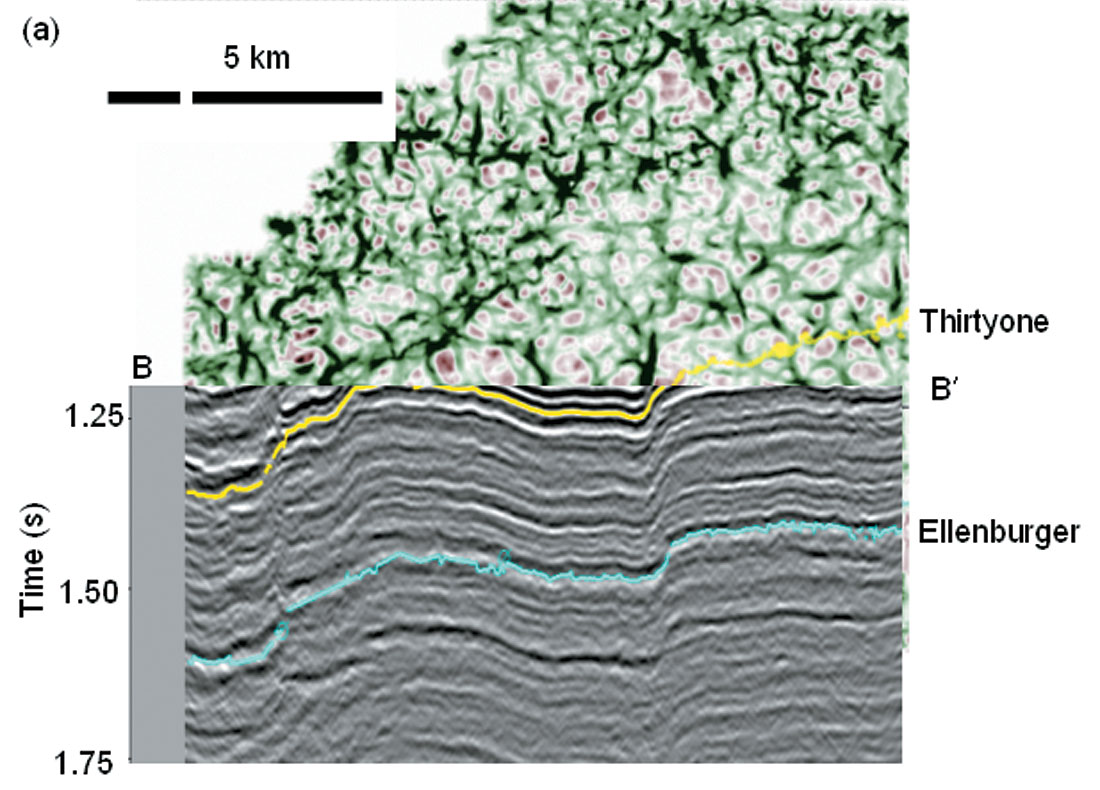
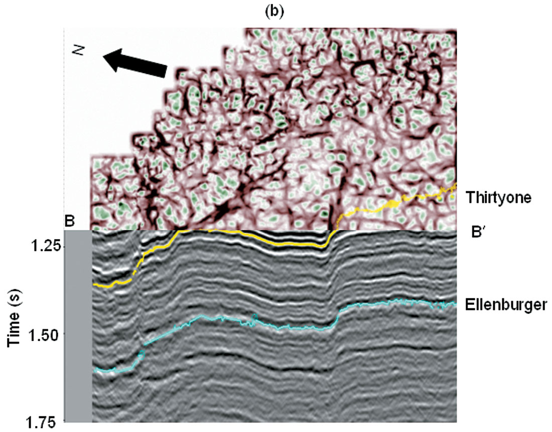
This example is drawn from a survey over the Central Basin Platform of West Texas, USA. The major production in this area is from the Devonian age Thirty-one Formation, which is a chert deposit carried from the shelf in the North by turbidity flows into this deeper part of basin. The reservoir is highly compartmentalized and is enhanced by fractures. In Figure 10a we show an image of the most-positive curvature extracted along the yellow Thirty-one Formation horizon posted on the vertical slice through the seismic data. In Figure 10b we display an enlarged view of the seismic data corresponding to a producing part of the reservoir indicated by the green box in Figure 10a. Green arrows indicate synclinal and red arrows anticlinal features within this structural high. In Figure 11 we display the time/structure map of the yellow Thirty-one formation pick shown in Figure 10a, as well as the corresponding coherence extraction (horizon slice through the coherence volume).
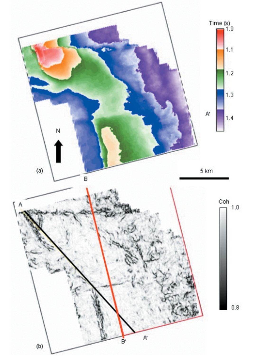
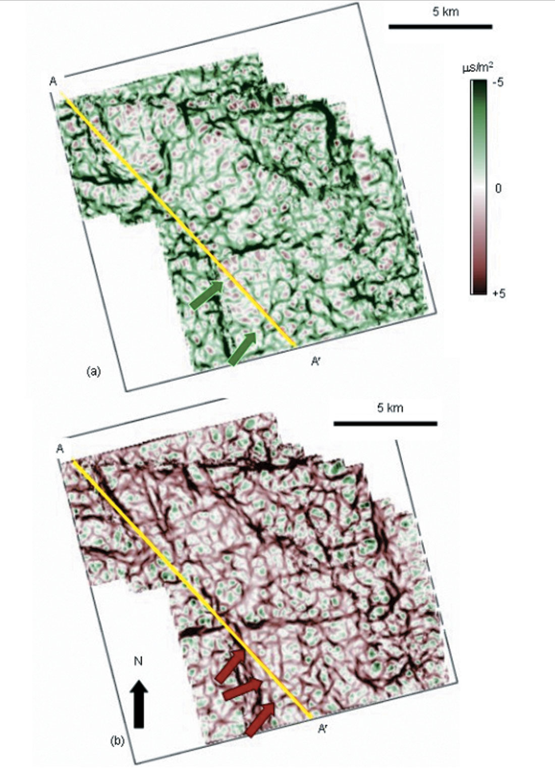
In Figure 12 we show corresponding horizon slices through the most-negative and most-positive curvature volumes. Green and red arrows correspond to those shown in Figure 10b. Note that this subtle warping seen on the vertical seismic can be carried along the entire horizon, providing constraints on the paleo stress environment and possible fractures. The coherence extraction is relatively featureless over the zone of interest while the curvature volume is not. This observation reinforces our major point that coherence and curvature volumes are different because they are measuring different attributes of the input seismic volume. In particular, curvature shows subtle (unbroken!) flexures not seen by coherence because coherence is sensitive only to lateral discontinuities. In contrast, we show images in Figure 16, where coherence will delineate channels and (in the absence of differential compaction) curvature will not. The curvature computations are volumetric rather than along a surface, which we illustrate in Figure 13 where we show time slices at 1.0 s through the most-negative and positive curvature volumes, where the posted yellow picks correspond to the intersection with the structurally deformed Thirty-one Formation. To more explicitly illustrate the correlation of these curvature computations to the original seismic data we display the seismic data, coherence, most-negative curvature, and most-positive curvature in Figures 14 and 15. These curvature images provide the interpreter with a means of mapping local highs (domes) and lows (bowls) as well as carrying subtle flexures across the entire survey.
Curvature versus coherence
Seismic attributes, including RMS amplitude, spectral decomposition, and geometric attributes are all computed in a vertical analysis window and remove much of overprint of the seismic wavelet from the image. The polarity of a channel reflection depends not only on the impedance of the channel fill (which changes within the channel system) but also on the impedance of lithologies that underlay and overlay it. Attributes that remove the seismic wavelet generate images that are more visually consistent to the interpreter when seen on map view. Attribute vertical analysis windows on the order of the dominant period of the seismic data also improves the signal-to-noise ratio of the image by stacking the information content of similar time slices together. However, vertical analysis windows much greater than the dominant period run the risk of mixing the uncorrelated information from overlying and underlying strata.
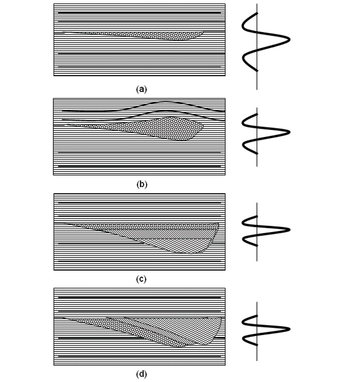
In Figure 16 we present three alternative models of how a channel may appear on different seismic attributes. Figure 16a shows a thin, flat-topped, channel below the tuning thickness. We observe that there will be no change in seismic waveform across this event, such that it will not be seen by coherence. However, the channel will be seen by RMS amplitude (and other energy measures), spectral decomposition, and coherent energy gradients. Figure 16b shows a thin channel that has undergone differential compaction. This channel also will not give rise to a coherence anomaly, will be seen by attributes sensitive to amplitude, but since it deforms the (thicker) sediments above it, will now be seen as a most positive curvature anomaly. Figure 16c shows a thicker channel, above thin bed tuning. The right side of the channel will be seen by coherence since the waveform of the composite reflection will change abruptly. The left side of the channel will be seen where it cuts an underlying reflector. The gentle taper will in general not be seen by coherence since the change takes place over a lateral area larger than the analysis window. The reflection from the bottom of the channel may be broken due to lateral varying impedance and may not generate an accurate estimate of geologic dip. This channel will probably not be seen by curvature attributes. Finally, Figure 16d shows a thicker channel that is aggradational in form. It will be seen by our full suite of attributes. More details can be picked up from Chopra and Marfurt (2006).
Curvature attributes for well-log calibration
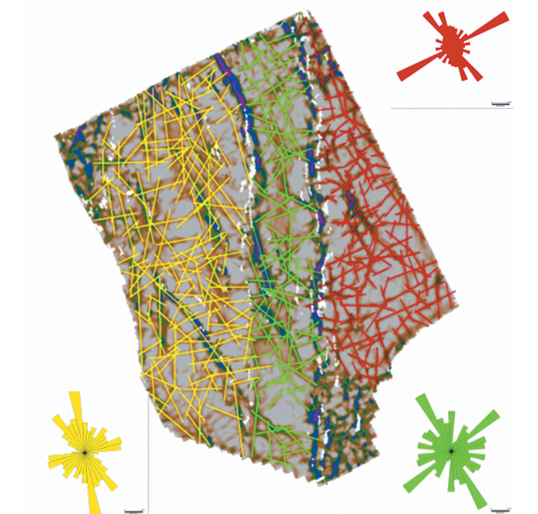
Figure 17 shows a phantom horizon slice extracted from the most-negative curvature volume at a level 120 ms below the horizon shown in Figures 4 and 9. The ability to display curvature along time slices, phantom horizon slices, and stratal slices that have not been explicitly picked is one of the major advantages of volume-based over horizon-based curvature computations. The individual lineaments in the three compartments formed by the two main faults running north-south have been tracked in three different colors. The orientations of these lineaments in the three compartments have been combined in the form of rose diagrams shown therein, retaining the color of the lineaments. These rose diagrams can be compared with similar diagrams obtained from FMI (Formation Micro-Imager) wells logs to gain confidence in calibration. Once a favorable match is obtained, the interpretation of fracture orientations and the thicknesses over which they predominate can be trusted for a more quantitative analysis, which in turn could prove useful for production from reservoirs.
(Data courtesy: Arcis Corporation, Calgary).
Conclusions
Curvature attributes are a useful set of attributes that provide images of structure and stratigraphy that complement those seen by the well-accepted coherence algorithms. Being second order derivative measures of surfaces, they can be quite sensitive to noise. Picks made on zero-crossings (on the quadrature of the data if appropriate) are in general less noisy than those made on peaks and troughs. Additional noise can be suppressed by iteratively running spatial filtering on horizon surfaces. Mean filters seem to do a satisfactory job and help enhance long-wavelength curvature features that may be difficult to see on the picked horizon itself. Median filters sharpen discrete horizon discontinuities such as faults. For the datasets under study, strike curvature, shape index, most-positive and most negative curvature offered better interpretation of subtle fault detail than other attributes. Volume curvature attributes provide valuable information on fracture orientation and density in zones where seismic horizons are not trackable. The orientations of the fault/fracture lineations interpreted on curvature displays can be combined in the form of rose diagrams, which in turn can be compared with similar diagrams obtained from FMI (Formation Micro-Imager) wells logs to gain confidence in calibration.

Acknowledgements
We would like to thank Chuck Blumentritt of Geotexture Technologies, Houston, for processing the volume curvature attributes and preparing the image shown in Figure 17. We also thank Arcis Corporation for permission to show the data examples and publish this work.


Join the Conversation
Interested in starting, or contributing to a conversation about an article or issue of the RECORDER? Join our CSEG LinkedIn Group.
Share This Article