Cost-Effective Seismic Exclusion Zone Mitigation Using Optimal Station Prediction (OSP) Method

For large seismic exclusion zones affecting numerous source and/or receiver stations, should all the stations within the exclusion be skidded or offset around the edges of the exclusion, or should select stations that provide the most geophysical and economic value be used instead? How do we quantify station value? Is it fold, offset/azimuth distribution of traces, the ability to infill offset vector tiles (OVT), also known as common offset vector tiles (COV), just the midpoint locations, or simply cost? In this article we detail the Optimal Station Prediction (OSP) method for optimizing station locations around exclusions that provide maximum subsurface coverage without wasting effort on excessively redundant stations.

Introduction

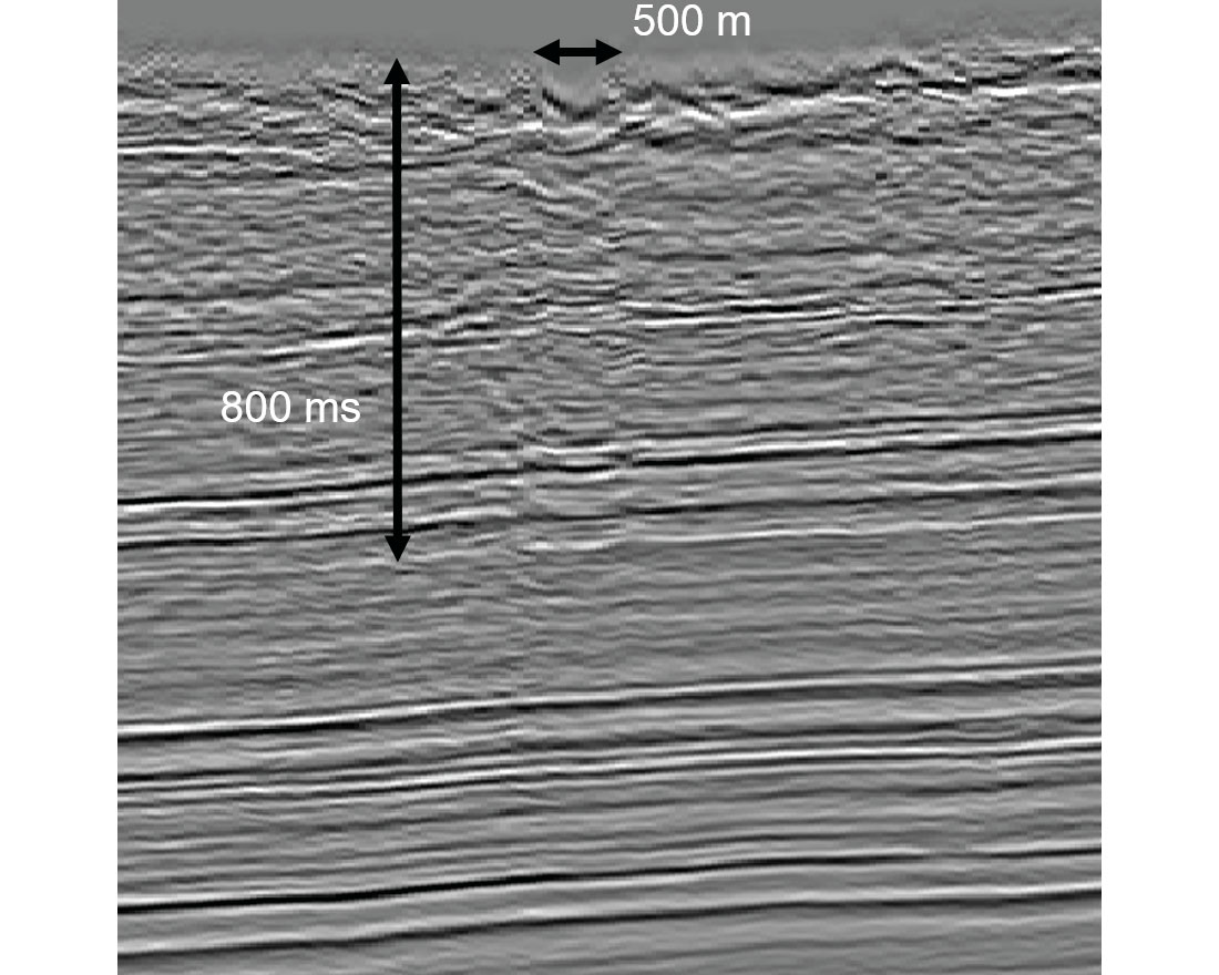
The impact of an exclusion on the seismic image is dependent on the width of the exclusion and the target depth. When a seismic survey is well designed for the target and appropriate mitigation measures are applied during exclusion modeling, surface exclusion zones have only a minimal impact on subsurface imaging. In Figure 1, the primary target (>1200 ms) is unaffected by a surface exclusion zone. However, the 500 m source and receiver gap affects both the structure and amplitudes of shallower horizons down to approximately 800 ms, and gaps in the data are apparent in the very shallow section. It is important that appropriate mitigation measures are applied when dealing with exclusion zones in order to minimize the impact of the exclusion zone on the data quality.

Exclusion Zones

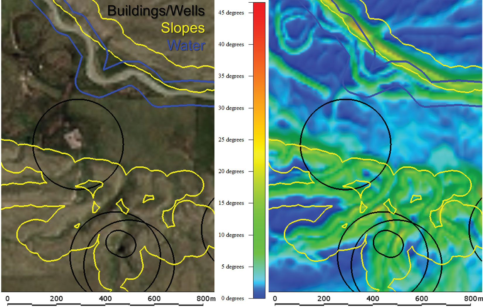
Exclusion zones in a seismic survey are typically due to natural obstacles such as rivers or steep slopes along river banks, environmental restrictions such as nesting sites and riparian areas, infrastructure such as buildings and pipelines, or permitting restrictions such as limited access or complete source and receiver lockouts. In sensitive environmental areas, the width of line cuts through forests may be reduced, which restricts the size of the source drill rig or vibroseis truck. In other areas, access may be limited to hand-cleared lines, restricting sources to those that can be carried into the area such as a hand auger or heli-drill. Figure 2 illustrates a combined natural (water & slopes) and infrastructure (buildings and water wells) exclusion zone.

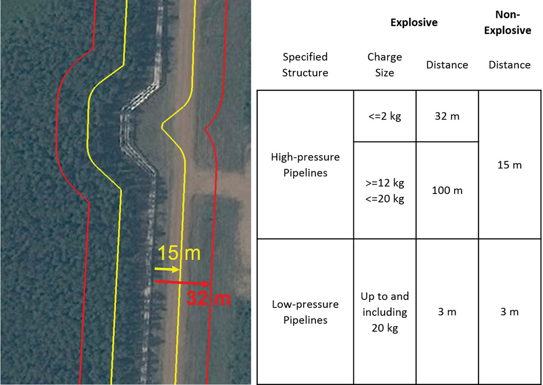
The size of an exclusion zone may also vary depending on the type of source used for the seismic survey. In areas around infrastructure, explosive sources have larger exclusion zones than non-explosive sources. For explosive sources, the size of the exclusion zone may also depend on the charge size (<2-20 kg). In Alberta, exclusion zones around infrastructure are determined based on the setback distances outlined in the Exploration Directive 2006-15, which describes explosive and non-explosive setback distances for buildings, pipelines, wells, etc. For example, the setback distance from a high pressure pipeline is 32 m for an explosive source with a charge size less than 2 kg, but only 15 m for a non-explosive source, such as vibroseis (Figure 3). In practice, these exclusion zones are actually larger as additional buffers ranging from 2 m to 10 m may be added in the field in order to avoid placing stations on the edge of an exclusion zone.

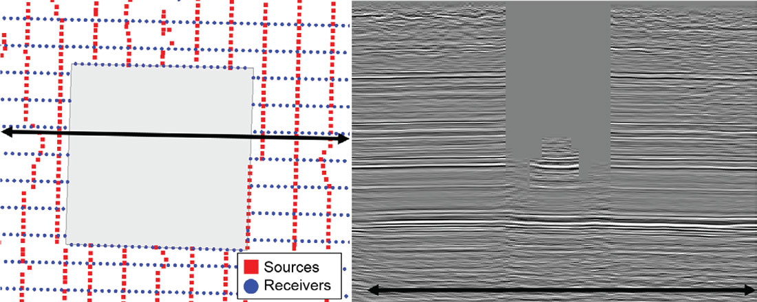
For large exclusion areas, such as permit lockouts, undershooting the exclusion zone may be a viable option if the target depth is greater than the width of the lockout. However, low-impact options such as utilizing road allowances, walk-only access, hand-drilled sources, nodal receivers and coarser grid parameters (i.e. 50% reduction in station density by increasing station interval across the exclusion zone) should also be considered. In areas where access is not possible, such as a permit lockout or a restricted environmental area, undershooting of the area may be the only option (Figure 4).

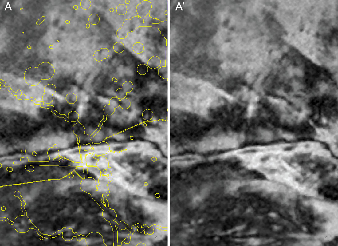
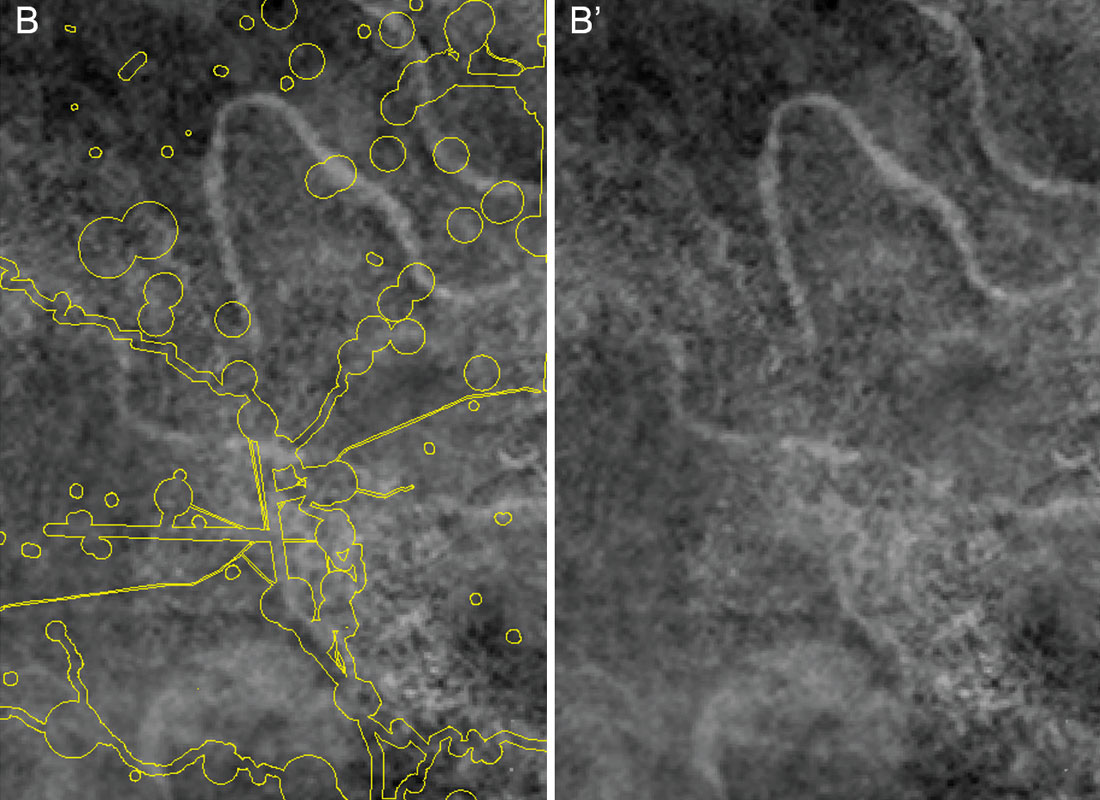
In areas with significant amount of infrastructure, overlapping exclusion zones may create large source gaps. Depending on the target depth and the number of exclusion zones within a seismic program, the effect of the exclusions on the final seismic data may be significant or negligible. In the following example, overlapping source exclusion zones result in a large area (1000 m x 2300 m) of source exclusions. At the primary target (>1200 m, >20 fold) imaging is not affected (Figure 5A). However, shallower in the section (<600 m, <12 fold) a channel structure visible on the north end of the processed time slice is partially obscured in the south due to the effect of the overlapping exclusion zones (Figure 5B).

Exclusion Zone Mitigation

Many exclusion zones can be identified and compensated for through surface modeling prior to field deployment. Natural exclusions such as waterways and steep slopes can be mapped or calculated from high– resolution imagery and/or LiDAR data. Source and/or receiver infill/ stub lines can be added to compensate for restricted access areas and lockouts identified during permitting. Infrastructure such as surface pipelines, buildings, and powerlines may also be identified from imagery and modeled around, but these exclusions, along with buried utilities/pipelines, need to be located in the field to ensure accuracy. For repeated surveys, such as 4D, exclusion zones may have changed from the previous survey – new pipelines and well pads may have been added. In these cases, exclusion zone mitigation not only needs to account for the missing ray paths, but also needs to focus on the offset and azimuth distribution of the missing traces.

For exclusions only affecting sources (or only affecting receivers), reciprocity can be used to recreate source-receiver ray paths affected by an exclusion zone (Vermeer, 2012). For example, if a source is missing due to an exclusion, locating a receiver at the excluded source location and then acquiring sources at all receivers that would have formed part of the source patch replaces all the missing source-receiver traces with the reciprocal receiver-source traces. However, this method can be inefficient in practice since a survey with a 12 line by 80 station (960 channel) patch would require an additional 960+ source points.

Common mitigation methods include (1) offsetting (crossline movement) and skidding (inline movement) stations around exclusions (Cordsen, 2000), (2) adding infill or stub lines (Millis & Crook, 2012), and (3) acquiring a survey with mixed source types and sizes (explosive and non-explosive) to reduce the size of exclusion zones. The common practice of acquiring every theoretical point no matter where it is skidded or offset can result in the acquisition of redundant data that may be discarded during processing. Without planned mitigation of exclusions through surface modeling, in complex areas, sources may be grouped around exclusions resulting in adjacent stations and duplicate ray paths within bins.

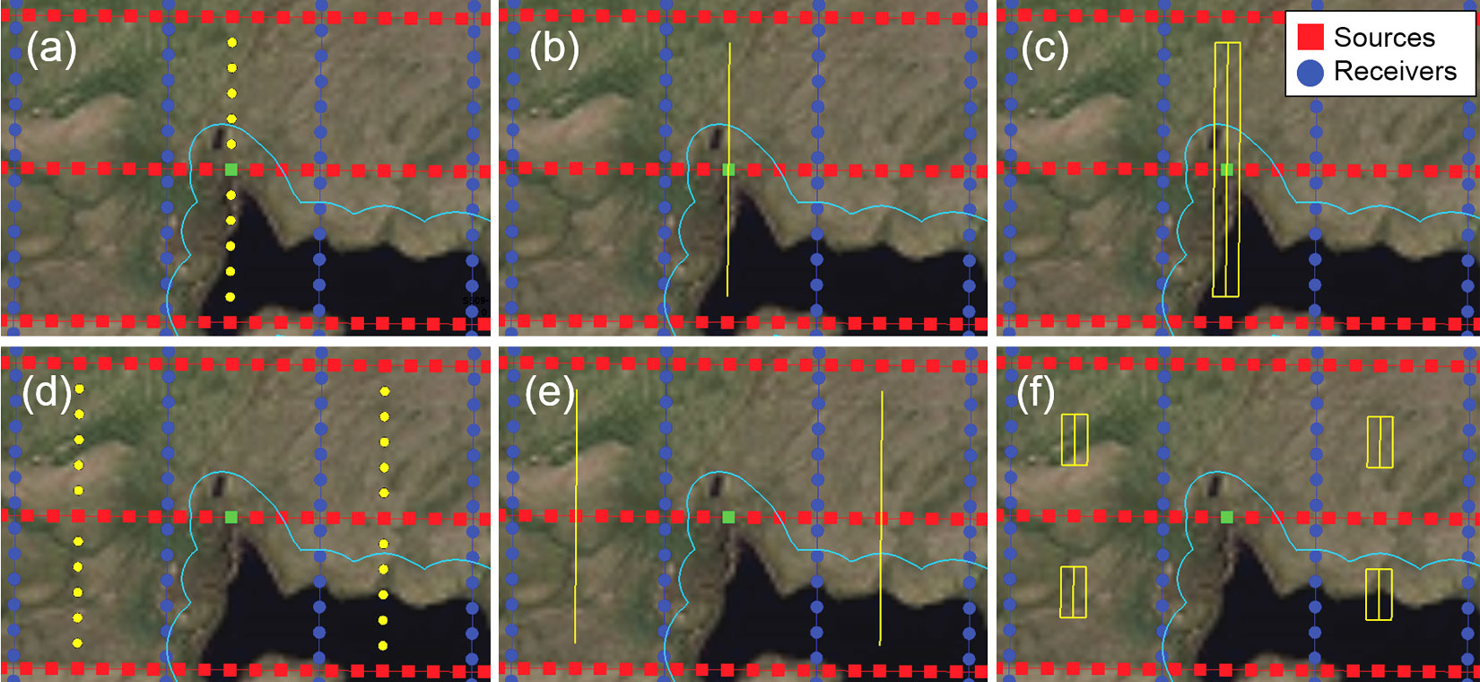
Standard source skid and offset procedures are based on the assumption that receiver stations remain at or very near theoretical locations. These procedures may involve moving stations within a radius of ½ a station interval, offsetting stations crossline from ¼ up to ¾ of a line interval, skidding a station inline one station interval (never recommended as this causes significant fold striping), or skidding a station inline by one line interval and then offsetting the station crossline by either a station interval or ½ a line interval. These various methods are illustrated in Figure 6.

Optimal Station Prediction

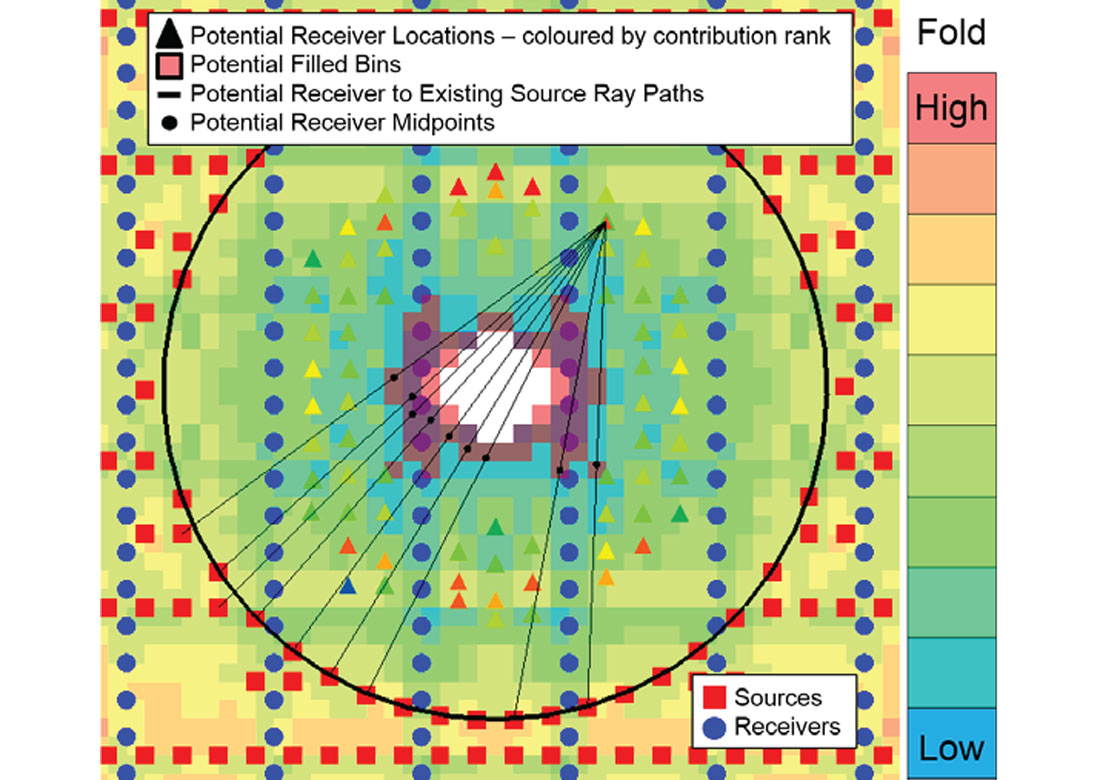
Source skid and offset guidelines work well when receiver stations remain within ½ of a station interval of the original theoretical grid. However, when receivers are moved off of the original theoretical grid, source-receiver ray paths are changed and the resultant midpoints no longer occupy the same bins (Millis, Caulfield & Crook, 2014). In areas with multiple, overlapping and/or large exclusion zones, standard skid and offset procedures may fail and an optimal station positioning method is recommended. In this method, initially discussed in Optimal restriction modeling: a new approach to station positioning (Millis & Crook, 2013), source and receiver pairs are modeled around exclusion zones to determine optimal placement based on offset, azimuth and fold requirements (Figure 7). In the following examples, we show an improved method, Optimal Station Prediction (OSP), based on an optimization that utilizes unique offset, azimuth or stacked OVT fold and focuses on target offsets.

When the diameter of an exclusion zone is greater than the target offset (i.e. mute at target or offset at target required for attribute analysis), skidding every source station within the exclusion zone that can’t be offset and/or adding receiver infill lines at half the line interval does increase the fold within the exclusion zone, but these station replacement methods result in redundant traces and significant fold halos around the exclusion zone. Additionally, these methods do not prevent gaps in the data. Rather than replace every station and end up with a significant number of traces that may be discarded in processing due to redundancy, the optimal station locations can be predicted based on target offset and azimuth requirements.

Examples

In the following example, a source exclusion with a diameter larger than the target offset has resulted in a low fold area with a data gap at the centre of the exclusion (Figure 8). This exclusion could be a water well with a 180 m explosive buffer affecting target offsets of 300 m (exclusion zone diameter = 360 m) or an 1800 m diameter source lockout affecting target offsets of 1500 m. Since no combination of source and receiver station will infill this gap, should all source stations that cannot be offset outside of the gap be skidded and acquired or should select stations that provide the most value be skidded?

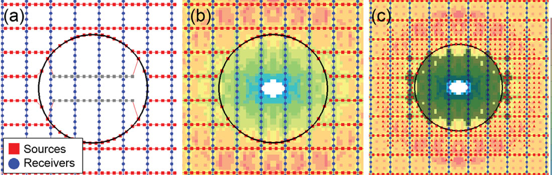
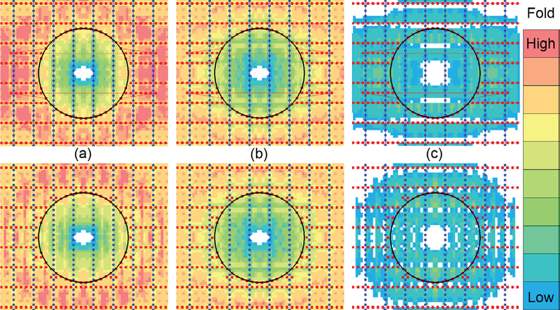
Figure 9 illustrates the result of skidding all 28 stations outside the exclusion vs. optimally positioning only 18 of the 28 stations outside the exclusion and excluding the rest. Optimizing the station locations based on azimuth and offset requirements and only selecting the most valuable ones results in less of a fold halo, more even OVT (Offset Vector Tile) fold and less redundancy in the offset vector tiles. Additionally, this method provides cost saving benefits since only 18 stations are needed.

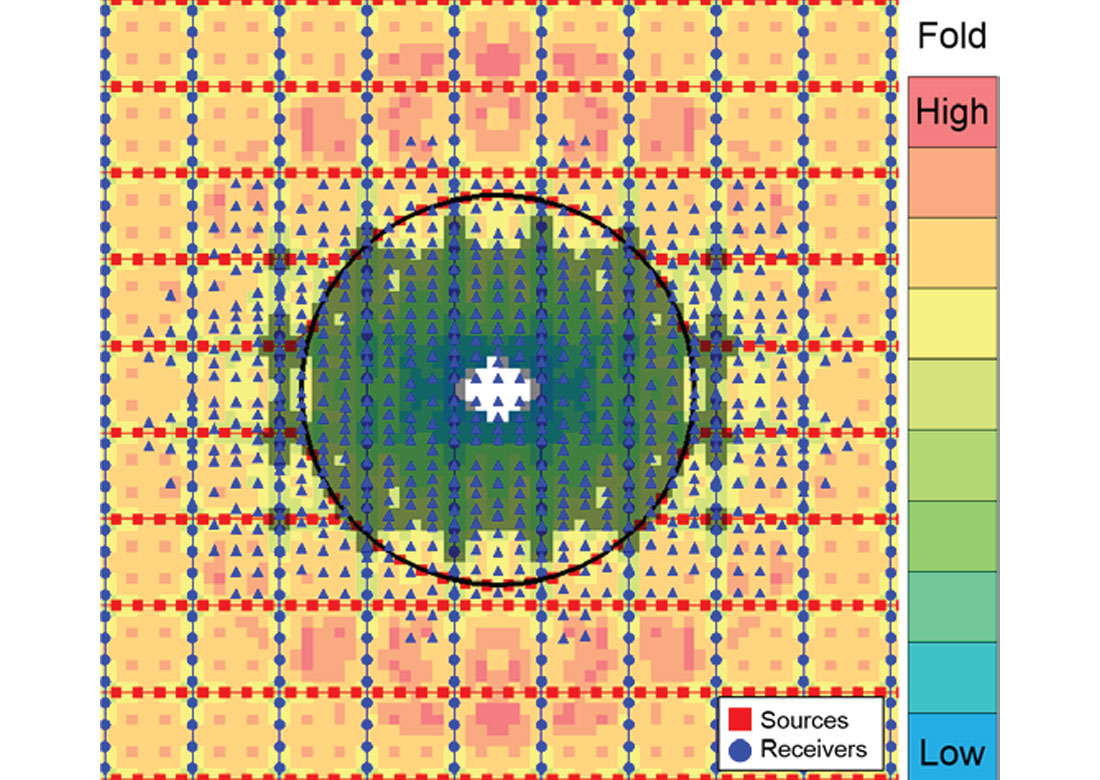
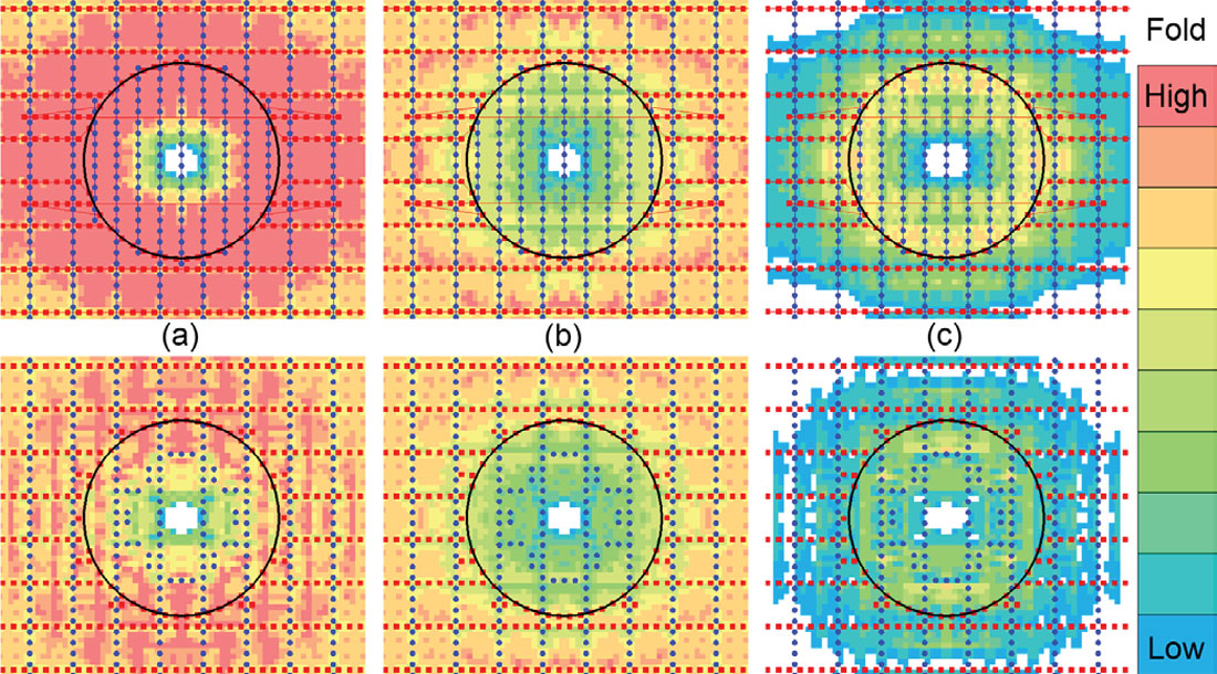
This method can also be used to optimize receiver infill locations. Although the data gap cannot be completely filled by adding infill receiver lines (Figure 10), the fold distribution within the exclusion zone can be improved. Results for receiver infill lines are similar to those obtained with adding source skid lines (Figure 11). In this case, twenty-six optimized receiver locations provide more benefit with less redundancy than eighty infill receiver stations placed at half the receiver line interval.

Both these examples are based on a theoretical circular exclusion. In the following example, we examine a real-world situation involving optimizing hand drilled source stations near a river exclusion zone. In this example, mechanical equipment is not permitted within the river valley. Therefore, any sources near the river will need to be hand drilled.

Skidding and offsetting every source station out of the river buffer will result in a significant amount of hand drilled source points and be very costly. Receiver infill lines have been considered, but are time consuming to implement.

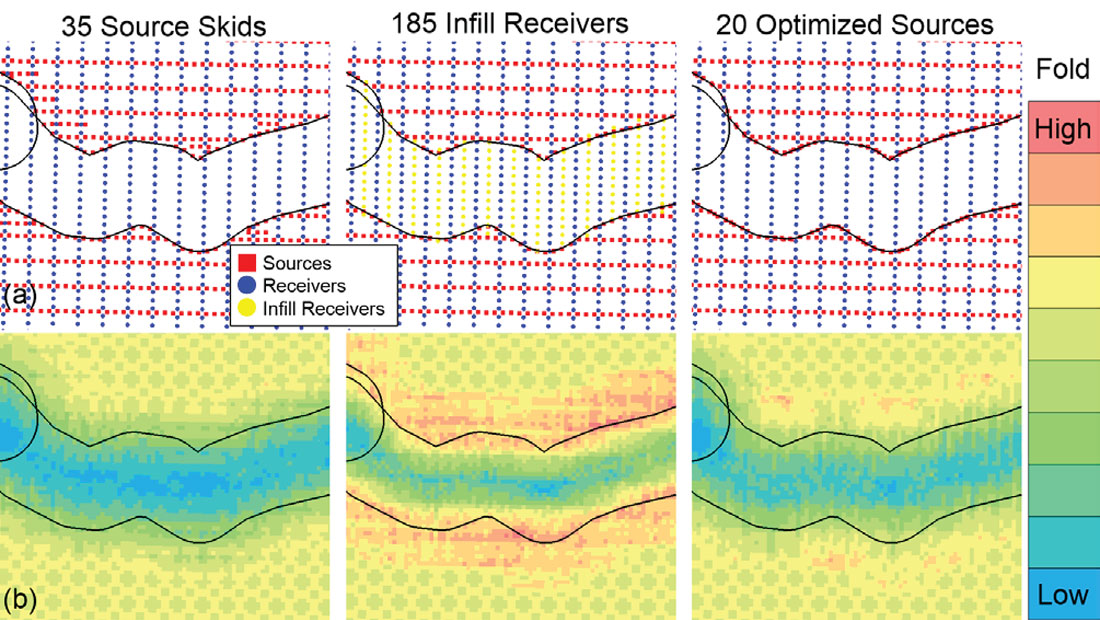
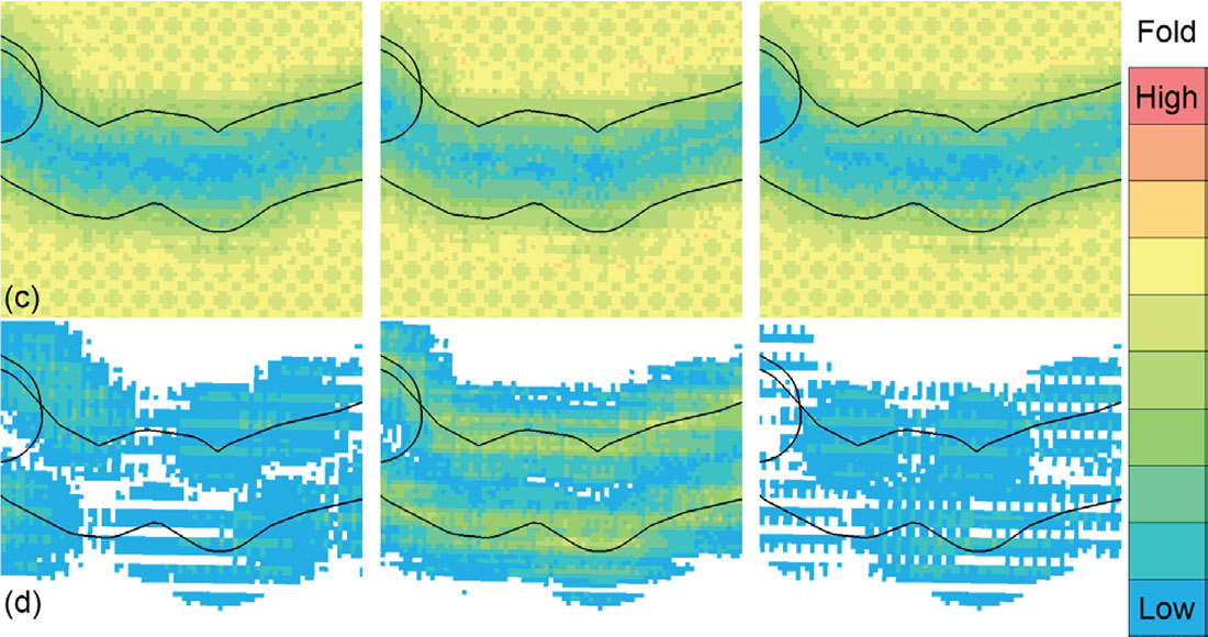
Figure 12 compares the results of skidding sources out of the river exclusion using skid/offset guidelines, adding receiver infill lines between existing receiver lines and utilizing the optimal station prediction algorithm to place a limited number of sources in locations providing the most value. In this example 35 source stations are skidded, 13 receiver infill lines are added every ½ line, resulting in an extra 185 receiver stations and 20 source stations are optimally placed along regular source lines to avoid extra line clearing. Results indicate that the optimally placed stations result in the best near offset distribution, the least fold halo and good OVT fold. Since station locations have been optimized onto existing and/or planned cut lines, significantly less line clearing is required for the optimized stations than for the skidded source lines or the infill receiver lines.

Conclusions

Most seismic programs are affected by exclusion zones. However, the effect of an exclusion zone on seismic data quality depends on both the size of the exclusion zone and the depth of the target. For surveys with shallow targets and/or large exclusion zones the imaging below the exclusion zone may be compromised. When exclusion zones affect both sources and receivers, undershooting may provide some benefit, but only if the exclusion width is less than the target offset. Common methods for dealing with exclusion zones, such as skidding and offsetting source stations, provide some benefit, but only when receiver stations remain within ½ a station interval of the original grid or vice versa for receiver offsets. A better method is to optimize station locations based on azimuth, offset requirements and avoiding redundancy in offset vector tile (OVT) fold. This Optimal Station Prediction (OSP) method can be used to selectively place only the most beneficial stations around an exclusion zone, providing a cost-effective method to acquire data in areas with numerous exclusion zones.

Acknowledgements

We would like to thank Explor for permission to show the data, SeisWare International Inc. for the interpretation software, and Cameron Crook at OptiSeis Solutions Ltd. for his contribution.