Comparisons of Geophysical and Medical Imaging

Geophysical and medical imaging are of great importance to society. In the case of geophysical imaging, we record waves passing through the Earth to image the Earth’s interior in search of anomalies to help in the exploration for petroleum and minerals. In the case of medical imaging, we image the interior of the human body in order to diagnose undesirable anomalies. Both imaging methods are done prior to invasive procedures. In the case of producing natural resources, geophysical imaging is done prior to costly drilling. In the medical case, imaging is generally prior to surgery.

Geophysical and medical imaging have their similarities and differences other than the fact that in the case of geophysical imaging we hope to discover anomalies whereas in medical imaging, we hope to not find anomalies. In this article, we hope to compare and contrast these imaging methods.

A good place to start this comparison is in the field of tomography. We examine seismic tomography and computer-aided tomography (CT scans). The word “tomography” is derived from the Greek word “tomos” meaning cut or slice and “graphos” meaning drawing. Thus tomography is based on the idea that an observed data set consists of line integrals along rays (i.e. projections) of some physical quantity. The goal of tomography is to reconstruct a model of a desired physical quantity (such as wave velocity) such that the model response agrees with the wave measurements.

Geophysical Tomography

We start with a discussion of geophysical tomography, specifically seismic tomography. Much of this discussion is an abbreviated form of papers by Bording et al. (1987) and Lines (1991).

In seismic tomography, we estimate a seismic velocity model of some part of the Earth’s subsurface such that the modeled traveltime agrees with the observed seismic traveltimes. If v(x,z) is the 2-D velocity field, s(x,z)=1/v(x,z) is the slowness or reciprocal velocity, and dl is the differential distance along the ray, the modeled traveltime associated with a given ray in a two-dimensional case is given by:

If t(data) is the observed seismic traveltime for a given source and receiver location, we desire a slowness field s(x,z) that will minimize the difference between the observed and modeled traveltimes, usually in a least-squares sense. That is, we minimize an objective function:

by adjustment of s(x,z).

Consider the geometry of ray propagation as shown in Figure 1. Here D_ij represents the distance of the ith ray in the jth velocity cell. If we minimize S to by setting 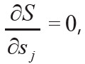we obtain a set of linearized equations given by:

Here Δt is a vector of traveltime differences, t(data) – t(ray), D is the matrix of ray distance values, D_ij , and Δs is the vector of slowness adjustments that will minimize S.

At first glance, equation (3) would appear to be a linear relation between traveltime differences and slowness. However, due to Snell’s Law and Fermat’s principle, rays bend to minimize traveltime and D_ij is dependent on slowness. Hence, for variable velocity fields, the problem is nonlinear. Solutions for slowness (and hence velocity) will require iterative solutions to equation (3) in which Δt is monitored and eventually minimized through iteration to an acceptable value.

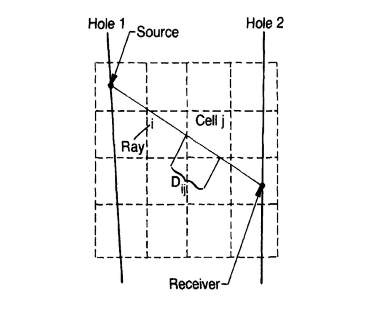
The seismic traveltime tomography problem is nonlinear since rays are generally not straight. Sources and receivers are generally confined to the surface of the earth or to boreholes, and therefore the source-receiver illumination of the subsurface is restricted. The velocity derived from tomography is often used in subsequent imaging of the Earth’s subsurface in depth migration. Nevertheless, velocity tomograms are useful in delineating subsurface geology as shown in Figures 2a and 2b from Lines (1991). Figure 2a shows a velocity tomogram from a cross-borehole experiment in which transmitted traveltimes from borehole sources to borehole receivers were used in equations in (3).

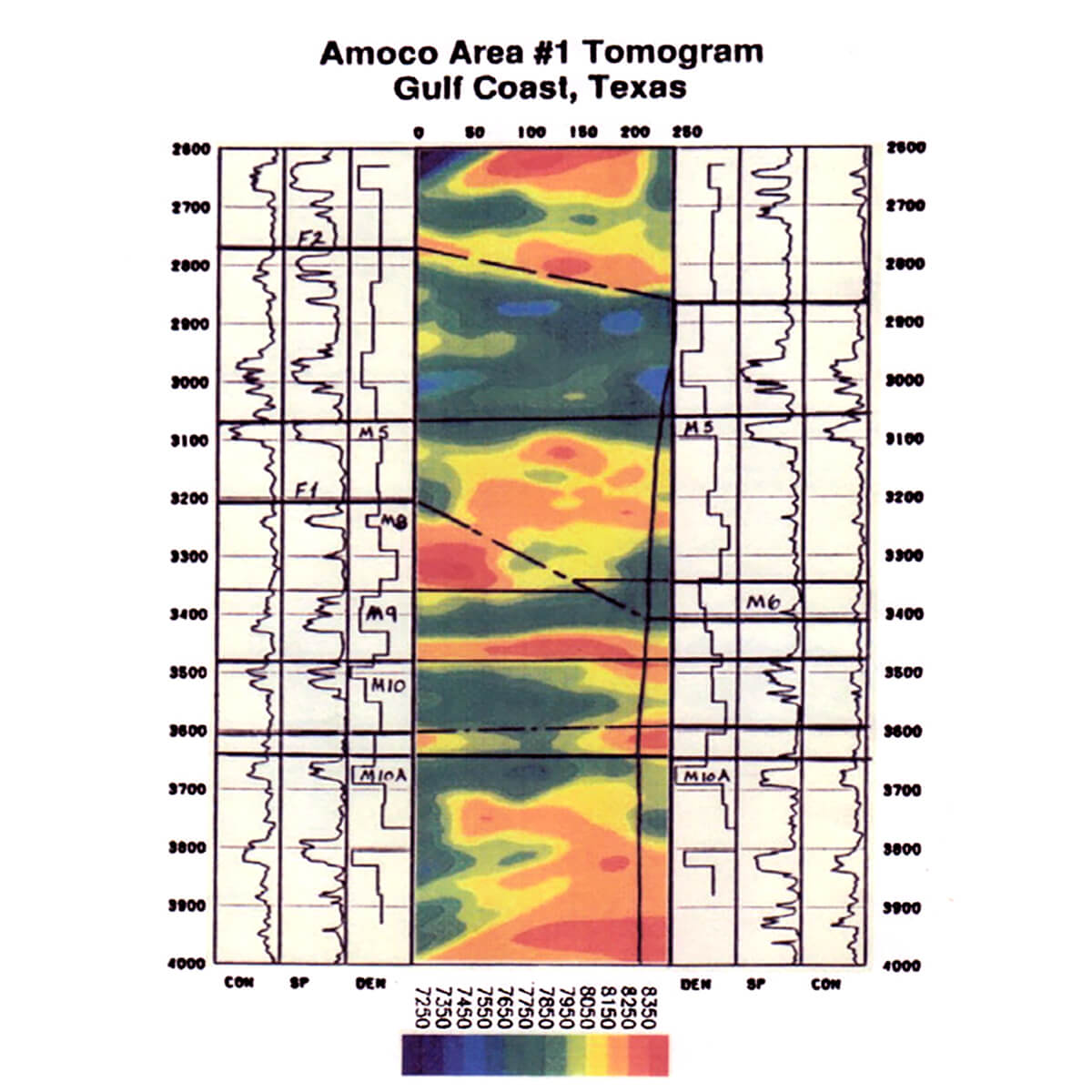
Figure 2b, also from Lines (1991) shows the velocity tomogram for a Gulf of Mexico salt intrusion that was obtained by using reflection traveltimes for the equations in (3). In this case the velocity tomogram was superimposed on a depth migrated seismogram which used these velocities in the depth conversion. The salt intrusion has a much higher velocity of about 4500 m/s ( or 14,750 ft/s), as indicated by the orange and red colours, than the surrounding sediments which have a velocity of about 2500 m/s (or 8200 ft/s), as indicated by the green colours.

Seismic traveltime tomography has been widely used in velocity estimation for seismic data processing and depth imaging.

Medical Tomography

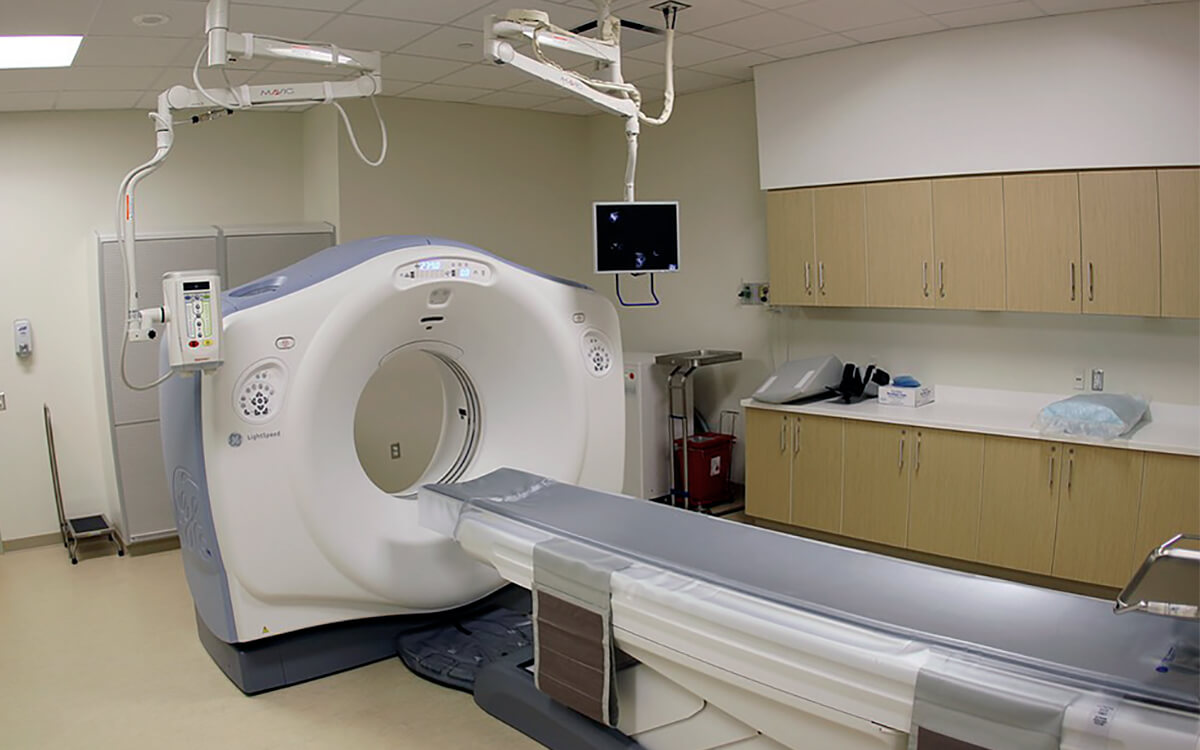
Medical tomography (CT scans), on the other hand, involves a much more controlled linear experiment with a source-receiver aperture that spans 360 degrees. The CT scan waves are X-rays, which can generally be considered to have straight ray paths, meaning that the problem is closer to being a linear one. Instead of evaluating wave traveltimes as in seismic tomography, the CT experiment deals with the decays of X-ray amplitudes in propagation through the human body. Figure 3 shows a diagram of the CT scan equipment in a photo from Wikipedia (daveynin from United States – New UPMC East Uploaded by crazypaco). The patient is inserted inside the donut shaped apparatus and X-rays are transmitted from source to receivers on the other side of the apparatus.

The line integral in this situation is similar to equation (1) but involves the attenuation coefficient, α(x, z) rather than slowness s(x,z). This can be viewed as a linear system since the rays are straight and equation (1) for traveltimes can be modified to be equation (4):

where 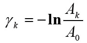is the integrated attenuation, where A_k is the amplitude at the end of the ray and A₀ is the initial amplitude at zero distance (reference: Dines and Lytle, 1979).

This will result in a set of linear equations in (5) that are similar to (3).

These equations in (4) and (5) for attenuation CT scans generally have a complete aperture, and different solution methods can be used – including those that use the projection slice theorem.

The Projection Slice Theorem – Medical tomography algorithms that would not work in geophysical tomography

Equations (1) and (4) are line integrals which represent the projection of 2-D functions along a path defined by dl. These projections can be related to 2-D Fourier transforms of the desired 2-D function, which in the case of CT scans is α(x, z). The projection slice theorem states that a 1-D Fourier transform in the wavenumber domain of the projection defined by (4) is equivalent to a slice through a 2-D Fourier transform of α(x, z) in a direction parallel to the projection line. In other words, the projection slice theorem describes how 2-D Fourier tranforms can be constructed by taking 1-D Fourier transforms of the projection. Then, in order to produce the desired image α(x, z) requires only that an inverse 2-D Fourier transform be applied. Using these Fourier methods requires a full 360 degree scanning of the object. While this method is fast and efficient in medical tomography where complete aperture scanning is done, it is not applicable to geophysical tomography where sources and receivers are on the Earth’s surface or in boreholes meaning that aperture scan is restricted.

Some Similarities Between Geophysical and Medical Tomography

While solutions to equation (5) in geophysical tomography would not use projection slice theorem principles, these equations can be solved by using ray tracing with solutions to large sparse linear systems of equations. There are geophysical case history examples where traveltime and attenuation tomography are used to sequentially solve the systems of equations in (3) and (5). Examples of these approaches include the research of Quan and Harris (1997) who compared velocity and seismic absorption tomograms in a West Texas oil field by using seismic traveltime and attenuation tomography approaches. Later in 2011, Vasheghani, Lines and Embleton used the Quan-Harris approach to produce absorption tomograms and then estimating oil viscosity tomograms from absorption tomograms through use of rock physics models. A more detailed version of the viscosity tomography approach is given by Vasheghani and Lines (2012). This approach could be very useful for reservoir characterization of heavy oil fields.

Electromagnetic Methods in Geophysical and Medical Imaging

Most of seismic exploration imaging uses reflections due to contrasts in acoustical impedance, where impedance, Z, is given by Z = ρv where is density and v is P-wave velocity. The reflection coefficient for normal incidence P-waves waves is given by the ratio of reflected amplitude to incident amplitude by:

If velocity variation is much greater than density variation, as is often the case for sedimentary rocks, the reflection coefficient is given by:

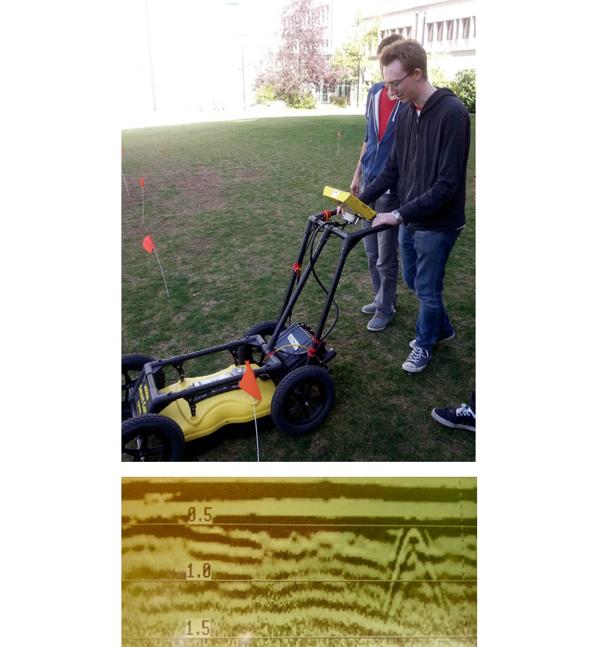
Not only is equation (7) a very useful equation in seismic reflection imaging, it is also useful in ground penetrating radar (GPR), where we deal with reflections of electromagnetic waves in the range of hundreds of MHz where wavelengths are in the 1-10m range (depending on the EM wave velocity, frequency and surface conductivity). GPR prospecting is widely used in near-surface measurements for engineering applications. GPR is usually simpler than seismic surveying and can be almost as simple as pushing an expensive lawnmower, and the record’s reflections and diffractions look very similar to seismic records. Figure 4 shows the operation of a 250MHz GPR unit (the Noggin) and an example of a GPR record.

A good review of GPR methods is given by Fisher, Stewart, and Jol (1992), who show that the reflection coefficient for GPR reflections is also given by equation (7). The EM velocities are given by where μ is magnetic permeability and ε is electric permittivity. Therefore for EM waves, the reflection coefficient for non-magnetic materials (where μ does not vary) is given by:

Equation (8) can also be expressed in terms of dielectric constants where the dielectric constant is a dimensionless quantity given by the ratio of a material’s electric permittivity to the electric permittivity in free space (Corson and Lorraine, 1962).

As noted above, GPR imaging is useful in geophysics for near-surface imaging down to depths of a few meters, and seismic imaging can be used down to depths of thousands of meters. For medical EM imaging of the human body, wavelengths must be smaller and are typically on the order of a few centimeters. For these purposes, high frequency EM waves known as microwaves are used with frequencies on the order of 1 to 10 GHz. Advancements in this area have been made in labs such as those of Dr. Elise Fear, in the Electrical Engineering Department at the University of Calgary.

A paper that describes this technology is an IEEE publication by Bourqui and Fear (2016) entitled “System for Bulk Dielectric Permittivity Estimation of Breast Tissues at Microwave Frequencies”. The paper describes an apparatus for measuring microwave transmission responses to estimate dielectric properties of the human breast in order to detect possible tumours. While the above GPR imaging uses reflections of radio frequency waves to estimate changes in dilelectric permittivity within the Earth, the medical imaging uses transmitted microwaves to image dielectric permittivity changes within breast tissues. Since the reflection coefficients, R, and transmission coefficients, T, are related by R+T=1, and since reflections are basically 2-way transmissions, it may be useful to utilize both reflections and transmissions. As pointed out by Bourqui and Fear (2016), the use of microwaves to assess dielectric properties of tissues may serve as a starting point for improved medical tomographic imaging.

Conclusions and Possible Future Research

The fields of geophysical and medical imaging have many similarities and differences. It is believed that geophysicists, electrical engineers, and medical imagers can learn from the advances in the others’ disciplines. The synergies should allow for advancements in both fields.

Acknowledgements

The authors wish to thank Dr. Steve Jensen for the excellent edits that he made to this paper.