Basic Geomechanics for Induced Seismicity: A Tutorial

We are increasingly accessing the earth’s crust to extract water, minerals, hydrocarbons, and geothermal energy and to dispose of waste CO₂ and liquids. All of these activities result in changes to the subsurface pore pressures either stabilizing a geological formation or nudging it closer to failure. Such failure becomes a concern for industry, regulators, and the public if it causes an earthquake that may be felt or, worse, result in damage. In this contribution we assume that this induced seismicity results from slip of a preexisting fault or other plane, the situation that may be expected to be most relevant in the Western Canada Sedimentary Basin.

Although the topic of induced seismicity has received a great deal of attention recently, this issue has been of concern for some time. Much of the early literature examined ‘reservoir induced seismicity’ (RIS) where in this context the reservoir means the lake that grows behind a dam. Geothermal energy requires that fluid volumes, typically much larger than encountered in hydrocarbon extraction, be produced and, usually, re-injected. To accommodate such volumes the ‘sweet spots’ for these projects are usually highly fractured rock masses in tectonically active areas.

Suckale [2009] has recently provided a comprehensive review of this topic listing 70 cases related to hydrocarbon production prior that time, but the prevalence of such seismicity is accelerating [e.g., Ellsworth, 2013]. Another relatively comprehensive review may be found in the report on induced seismicity sponsored by the U.S. National Academies of Sciences [NRC, 2013]. That said, in light of developments in both Canada and the U.S. even within the present year, this is a topic that is rapidly evolving.

Earthquakes of varying intensity have also been recorded in the Western Canadian Sedimentary Basin (WCSB) [Milne and Berry, 1976] and with the growth of hydraulic fracturing stimulation and the consequent re-injection of volumes of produced fluids. The most prominent event to date occurred near noon on March 8, 1970 Snipe Lake event (to the east of Valleyview, Alberta) with a significant magnitude m_b = 5.1 [Milne, 1970] resulting in intensity ratings as high as III (noticeably felt indoors) according to surveys mailed out to the public after the event. Milne tentatively suggested that this earthquake, occurring in an otherwise area of low seismicity, might be linked to fluid injection for enhanced oil recovery but the large uncertainties in the position of the event’s hypocentre do not allow for a definitive linkage.

A number of studies have also focussed on seismicity near Rocky Mountain House, Alberta where a number of M < 3.4 earthquakes were located beneath the Strachan gas field [Rebollar et al., 1982; 1984; Wetmiller, 1986] where statistical linkages between the rate of gas production and seismicity could possibly be explained using a time-dependent poro-elastic model [Baranova et al., 1999]. Seismicity in this area has diminished in recent years likely due to declining production rates associated with this mature field [Stern et al., 2013].

The best documented case to date, however, is that of Horner et al. [1994] who described the appearance of significant felt seismicity with the greatest magnitude of M 4.1 and with intensities of IV to V experienced from 1984 to 1993 near Fort St. John, B.C.. They carried out an extensive geomechanical analysis that strongly suggested that the high fluid pressures (25 MPa) injected and associated lowering of effective stresses could be responsible.

Studies on seismicity clusters continue to the present. Schultz et al. [2014] describe observations of seismicity associated with the Brazeau cluster near the Cordel waste water disposal well from which fluids are injected at depths of 3796 m to 3896 m. The level of seismicity, with events up to M = 4, correlates strongly with the monthly rate of fluid injection.

The most serious petroleum related seismicity, such as has occurred in Oklahoma, appears to be linked to disposal wells in which large volumes of fluids are injected over time periods of years. However, more recently induced seismicity has also been tied to hydraulic fracturing both in the Horn River Basin of NE British Columbia [BCOGC, 2012] and in the Fox Creek area of Alberta [Novakovic et al., 2014].

Clearly, such seismicity is of concern to industry, regulators, and the general public. All of the recent syntheses [CCA, 2014; NRC, 2013] suggest that we only poorly understand these phenomena and that more work is necessary in improving observations, better understanding the physics and geomechanics of in situ processes, and in developing accurate predictive models. In this contribution, we seek only to briefly review some of the more basic geomechanical aspects of induced seismicity according to the Coulomb frictional failure criteria. This entails an overview of the underlying definitions of crustal stress and pore pressure, the setting of the geometry of the failure plane within different co-ordinate systems, and discussion of how normal and shear tractions and pore pressure control slip stability. It must be kept in mind that this is the most basic of presentations, but I hope the reader will be able to use this contribution as a stepping stone to the more advanced literature and that it will help to motivate geophysicists to learn more about geomechanics.

Basic Concepts

In this short contribution we will only consider the slip along pre-existing planes of weakness in the earth as these will, generally, be more easily moved. A more complete presentation would also include a discussion of the rupture, or failure, of intact rock, the reader can find this material in many texts on rock mechanics. That said, planes of weakness are present throughout much of the crust. Figure 1 gives a number of examples in different locales in Alberta. They appear with different orientations as illustrated in the ultrasonic borehole televiewer imaging of a massive formation (Figure 1a), with parallel patterns of joints in an exposed argillite (Figure 1b), with direct evidence of slip along a plane through a core of Duvernay Formation rock (Figure 1c), and by the complex pattern of at least three joint sets in an exposure of the Milk River Formation sandstone (Figure 1d).

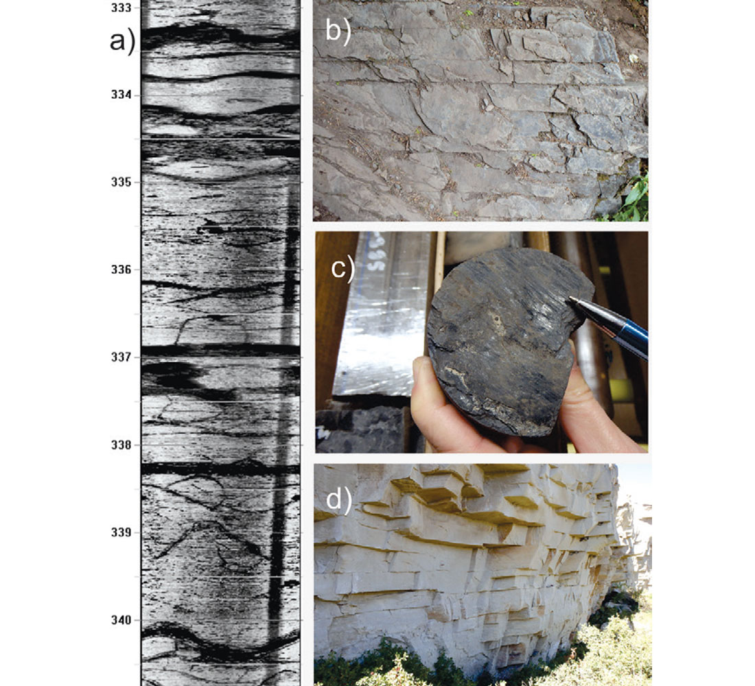
These images are mostly to demonstrate that various formations in the crust are often already broken and that there are often planes available for slip if the conditions are appropriate. Indeed, some workers believe the ubiquity of such features paradoxically keep the crust strong through continual failure and slip. The essential paradigm assumes that slip occurs on pre-existing plane of weakness once the effective stresses on the plane exceed the frictional forces across the fracture surfaces; and that is the “take-home” message. As usual, however, the devil is in the details and below I will review the relevant definitions and physics that controls such slip with discussions of the state of stress, the geometry of the problem, and the influence of pore fluid pressure and friction on stability.

State of Stress: Definitions

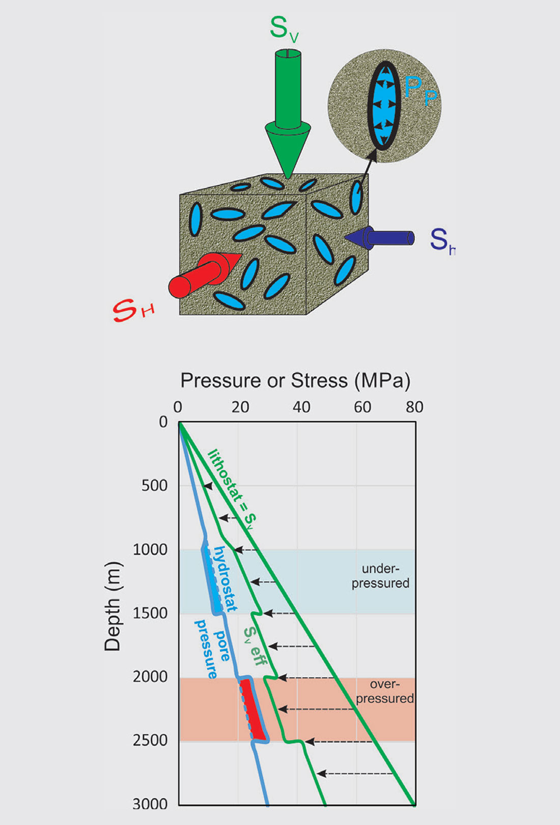
We nominally describe the state of stress in the earth in terms of the three principal total or confining stresses assumed to align with the vertical and two horizontal axes (Figure 1a). Along these axes are directed the lithostatic vertical stress _SV and the greatest and least horizontal compressive stresses S_H and S_h (see Schmitt et al. [2012] for more details of the inherent assumptions and limitations of this framework). S_V is the same as the overburden stress (and often called the lithostat) while S_H and S_h reflect the local tectonics, stress concentrations according to the elastic properties of the formation. It is crucial to understand also that the relative compressive magnitudes of these three define the three Andersonian normal, reverse (S_H ≥ S_h ≥ S_V), and strike-slip (S_H ≥ S_V ≥ S_h) faulting regimes. Note that in the examples to follow here we will assume a normal stress regime.

Many workers attempt to use sonic log measurements of Poisson’s ratio to calculate a horizontal stress magnitude but this should at best be only taken as a possible reference point. Using this can lead to error given that the relative values of the magnitudes between S_V, S_H, and S_h need not be constrained and, indeed, are key to determining the Andersonian faulting environment and the direction that a nominally tensile hydraulic fracture will propagate.

The pore fluid pressure P_P (Fig. 1a), or reservoir pressure in petroleum engineering parlance, is also a key parameter that cannot be ignored when it comes to failure. We delay discussion of this momentarily, and it will reappear when the concept of effective stress is introduced.

S_V necessarily increases with depth z (Fig. 1b) with progressively larger overburden loading. We also generally expect S_H and S_h to also grow (these are not shown for the sake of clarity). If the ground water has a density ρw, we also anticipate that the normal hydrostatic pressure is given by P_p = ρ_wgz. P_P(z) is often called the hydrostat and serves as a useful reference: formations in which the pore pressure is greater or lower than the hydrostat are, respectively, over- or under-pressured (Fig. 1b).

Pore Pressure and Effective Stress

This is a good point to introduce the concept of effective stress. For our purposes, the effective stress is simply:

where the subscript i = V, H, or h indicate any of the three principal (also normal) stresses. This is often also called the Terzhagi or the simple effective stress. It is important to note that the simple effective stress is that to be used for the failure of rock and the slip along pre-existing planes of weakness is not the same as the poro-elastic effective stress, in which P_P is modified by the Biot effective stress co-efficient [e.g., Detournay and Cheng, 1993; Wang, 2000] a parameter the inappropriate application of which has propagated through the literature and in practice (see Jaeger et al., [2007], pg. 98). In the remainder of this contribution, we take Eqn. (1) to be the one that defines the effective stress for failure or slip.

The corresponding S_Veff(z) also is shown in Fig. 1b. An interesting observation here is that S_Veff < S_V in the over-pressured zone but S_Veff > S_V in the under-pressured zone. At first site, one might think that because the effective stresses are greater in the under-pressured formation slip will occur there. This is not the case; slip is more likely in the overpressured regime with the lower effective stresses.

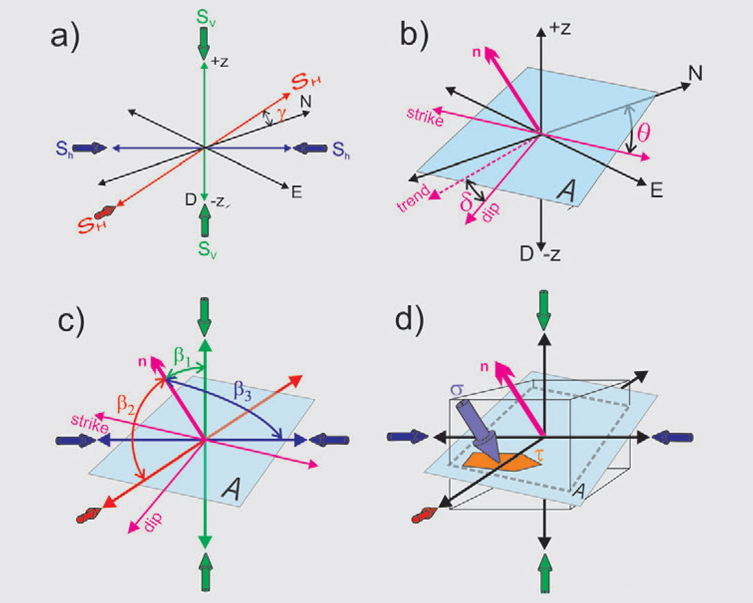
Before discussing this, it is crucial that the geometry of the problem be examined (Fig. 3). First, it must be remembered that the directions of the principal stresses are not generally aligned with our north-eastdown (NED) co-ordinate system [Allmendinger et al., 2012], in Fig. 3a the principal stress reference frame is shown rotated by an angle γ from geographic north. An arbitrary slip plane A, shown in Fig. 3b, is referenced to the geographic NED co-ordinates using the plane’s strike θ and dip δ angles; this plane may also be described by its surface normal n. In the principal stress co-ordinate frame it is more useful, however, to describe this same plane’s orientation in terms of the three angles β₁, β₂, and β₃ taken to n from the axes of the greatest, the intermediate, and the least principal compressive stresses, respectively.

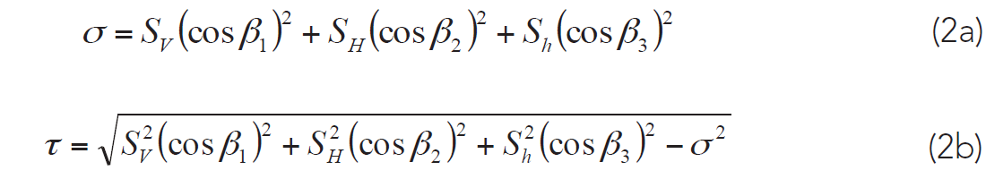
The key geometric issue is that the principal S_V-S_H-S_h stress state can be resolved into a traction (Fig. 3d), or stress vector that acts on A, this traction (not shown) can further be broken into a surface normal component σ (β₁ , β₂ , β₃) and a surface parallel shear component τ (β₁ , β₂ , β₃). σ is usually called plane’s normal stress, and within the context of the current discussion is also referred to as the clamping stress. Similarly, τ is the shear stress on the plane. Reducing the problem to σ and τ will simplify the analysis a great deal. These can readily be calculated using:

Visualizing the Stresses with Mohr Diagrams

It is useful to introduce the σ−τ space Mohr diagram [Parry, 2004], which is a longstanding tool used to visualize three-dimensional principal stress states. The three principal stresses SV, SH, and Sh appear as (σ,τ) points on the τ = 0 axis in the Mohr circle of Fig. 4a. The utility of the Mohr circle is that one may determine graphically the range of σ and τ for all the possible orientations of the potential slip plane A with normal n oriented at β₁ , β₂ , and β₃ . For example, the clamping and shear stress on our hypothetical plane A can be found at the intersection of the red, blue, and green-dashed circles each of which is the locus of possible (σ,τ) for each possible plane all of which are included in the blue shaded zones between the three Mohr circles. I leave it to the reader to investigate why the dashed circles launch from the 2β angles; this is important but not crucial to the following discussion.

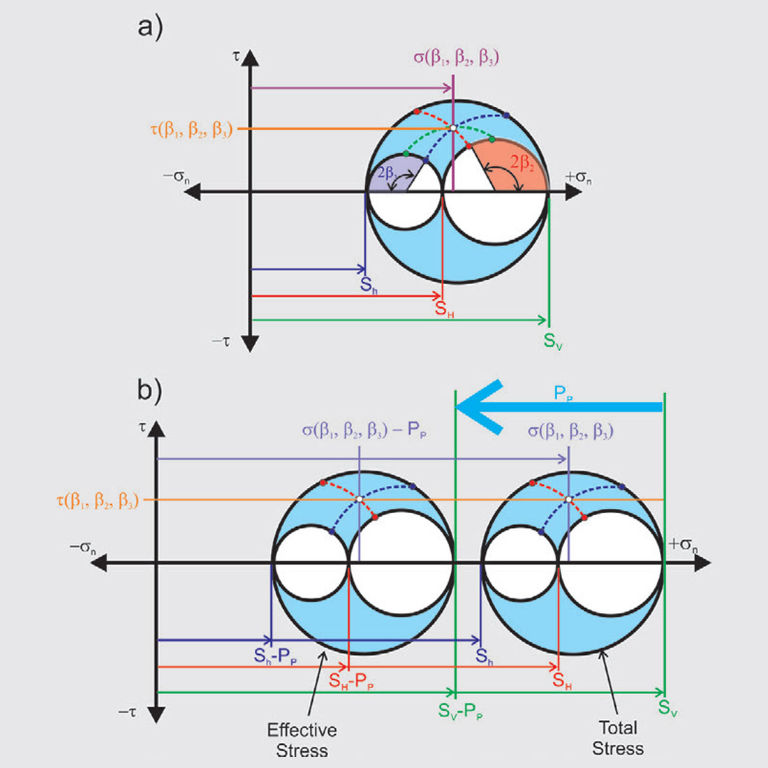
The state of effective stress, too, may be represented using the Mohr diagrams (Figure 4b). The effective stress relation of Eqn. 1 holds for any normal stress σ but does not influence the shear stress. Consequently, the effective stress Mohr circle is found by simply shifting the total stress Mohr circle to the left. Note that there shear stress τ is not changed; the P_P affects only the normal stresses.

Note that in this contribution we how the full Mohr circle representation includes the intermediate compression that for the normal faulting case presented here is S_H. Many discussions in the literature that focus on crustal failure consider only the difference between the greatest and least compression and show only the largest circle, these are usually concerned with motion on larger faults that are the orientations of which are generally assumed to be already optimally oriented [e.g., Sibson, 1990] or because of the simple lack of information on the intermediate stress value. In the case of induced seismicity, however, one would expect a wider range of smaller weakness plane to be available to slip and hence it is important to at least recognize the importance of the intermediate compression although this may not always be possible.

Rock Surface Friction

So far we have been able to represent the states of total and effective stresses on any potential plane of weakness, but this tells us nothing about whether a given plane will slip or not. We need to consider the role of friction in holding the rock masses welded to one another until the appropriate stress conditions are attained to produce slip (Fig. 5a). The Coulomb frictional criterion in which the slip plane remains stable as long as:

where C is the cohesion, a measure of the shear stress on plane A required to induce slip when the effective normal stress σ − P_P vanishes, and μ is the co-efficient of friction. Once τ exceeds this limit (Fig. 5b) the frictional forces are exceeded and slip can occur.

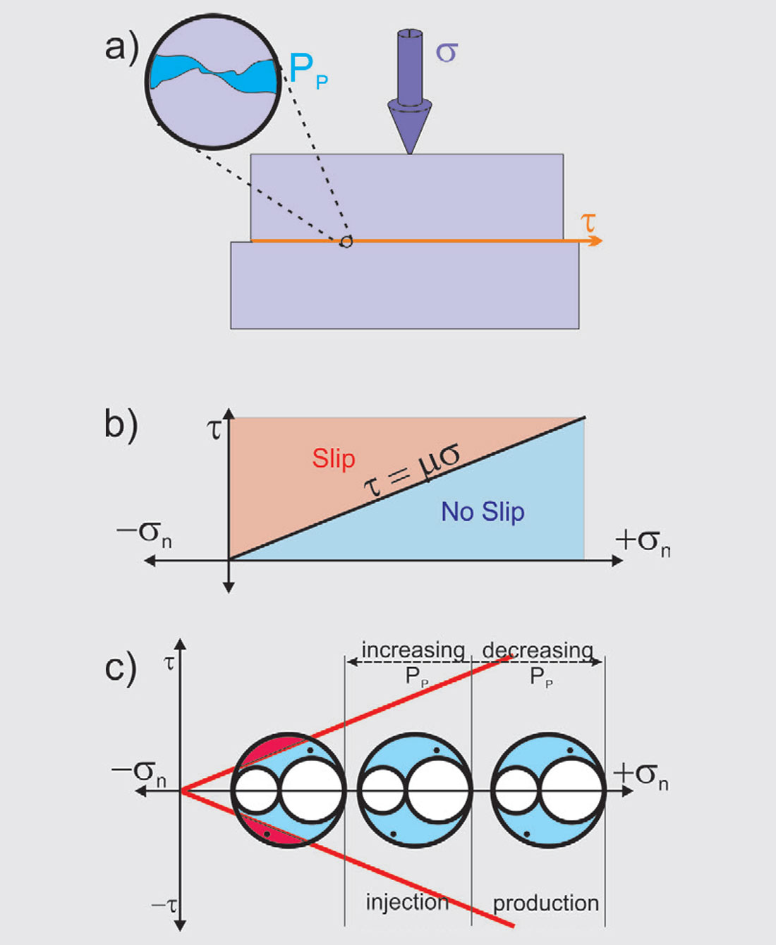
What values of μ should be used? Byerlee [1978] carried out an extensive series of friction measurements on a variety of rock types and suggested a value of μ = 0.85 for clamping normal stresses less than 200 MPa (≈ 29 kpsi) and μ = 0.6 at higher stresses to 2000 MPa. It is important to note also that μ is much lower for clay or fault gouge surfaces where values of μ of about 0.2 can occur. A good deal of evidence from quantitative crustal stress measurements often suggests that stability of the crust suggests 0.6 < μ < 1 [Townend and Zoback, 2000; Zoback and Townend, 2001]. It is also worth mentioning that there are more complex friction rules that can depend on the initial state and the length of time a given load had been applied [e.g., Dieterich, 1972] but this is beyond the scope of this introductory tutorial.

Stability of Slip Surfaces

All of these concepts come together in Fig. 5c. The central Mohr circle represents the virgin state of effective stress before P_P is perturbed. Note that two points are indicated in this Mohr circle, these represent two individual potential planes of weaknesses with differing orientations. The two red lines also fall along the loci of the Coulomb friction criterion of Eqn. 3 where, for the sake of convenience, we assume that C ≈ 0.

There are two important observations. First, consider the case in which fluids are produced from the formation such that P_P decreases. As already shown in Fig. 1b, this results in larger normal effective stresses as represented by a shift of the Mohr circle to the right. The allowable (σ,τ) values still all fall in the blue shaded region between the three, now shifted, circles, and away from the slip criterion lines. Consequently, decreasing P_P even further stabilizes the formation as no slip is allowed on a plane of any orientation.

Increasing P_P has the exact opposite effect. The effective normal stresses decrease with the new state illustrated by the set of Mohr circles shifted to the left. In this case the shifted circles intersect the slip criterion curve, and in Fig. 5c the area between this line and the circle has been shaded in red. This red area highlights the family of favourably oriented planes that lie above (or below for negative τ) the slip criterion line of Eqn. 3 and consequently will slip. That is, a plane of weakness is unstable if its orientation β₁ , β₂ , and β₃ is falling within the red zone.

Applying These Concepts

The application of these ideas is called a slip-tendency analysis [e.g., Morris et al., 1996]. For a given planar feature, ideally one would have knowledge of i) the principal state of total stress, ii) the orientation of the plane in the co-ordinate frame of the principal stresses, iii) the pore pressure, and iv) knowledge of an appropriate criterion for slip (i.e. usually the friction co-efficient). With this knowledge one can then determine if the plane will be stable or not as illustrated in Fig. 5c. A recent example of such a set of calculations in the Peace River area of Alberta to a series of faults located from legacy seismic data has recently been provided by Weides et al. [2014].

To conclude, it is likely that such stability analyses will become increasingly frequent in the future given the concerns associated with induced seismicity. Outside of the risk analysis aspects, carrying out these analyses too should help in identifying those joints or fractures that might also be most permeable. Doing all of this, of course, is going to require better knowledge of in situ stress states and pore fluid pressures. New frictional tests may need to be carried out on the rocks that are being subject to hydraulic fracturing because their high organic carbon and clay contents may influence the value of the co-efficient of friction. Finally, work will need to be carried out on locating potential slip planes whether they be faults appearing in 3D seismic volumes down to thin fractures that may be only be seen in core. Regardless, this provides exciting opportunities for geophysicists who are likely best positioned to be able to integrate all of the various kinds of data necessary.