Azimuthal Processing for Fracture Prediction and Image Improvement

Abstract

Oil and gas production from tight, fractured reservoirs (sandstones, carbonates, shales) has increased considerably as commodity prices have risen over the past 5 years. A common aspect of these hard rock targets is an oriented stress field and open fractures. P-wave seismic processing that can identify these variations in the subsurface and take advantage of them will produce sharper images and improved fracture predictions. The following paper discusses various azimuthal processing techniques used to identify azimuthal velocity anomalies and azimuthal AVO anomalies. These techniques can impact the final stacked image and the prediction of open fractures.

Introduction

Well data has long been a measure of fracture presence in tight-rock reservoirs. Borehole breakout, FMI measurements, and coring have provided clear indications of oriented stress fields and open fractures. Prospecting for fractures with the bit is an expensive and often unrewarding endeavor. Multicomponent acquisition, processing and interpretation may offer an opportunity for finding fractures with seismic but at an added time and financial cost compared to P-wave data. Early attempts to predict fractures with unmigrated P-wave data have been encouraging but the technique lacks spatial resolution. Sectored migration overcomes some of the limitations of operating on unmigrated data but often suffers from under-sampled azimuths in the input dataset resulting in noisy output. This paper discusses the use of a full azimuth Kirchhoff migration approach for detecting azimuthal velocity anomalies. The variation in velocity versus azimuth is a potential indicator of open fracturing. With the measured azimuthal velocity field one then can effectively pursue Azimuthal AVO anomalies as an additional fracture indicator. The workflow can be modified for a depth migration approach to address overburden velocity complexity (not discussed in this paper).

Understanding Fractures and Seismic

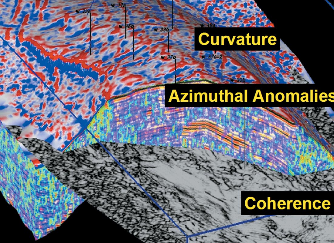
Natural fractures play a major role in determining the producibility of moderate-low permeability reservoirs. Intersecting fractures with properly placed vertical or horizontal well bores can provide access to greater reserves and provide for higher production rates. Fracture location, density, orientation and complexity will vary with the rock type and local stress. Field development requires a map-based understanding of fracture patterns. Seismic data offers an indirect measure of the effects of fracturing either through measuring shear-wave splitting (multicomponent acquisition and processing), azimuthal variations in P-wave velocity, Azimuthal AVO or post-stack techniques like Curvature Analysis, Coherence or Inversion. There is no single technique that works best all the time and a combination of the above is usually the best approach for gaining confidence in a fracture prediction (Figure 1).

Anisotropy

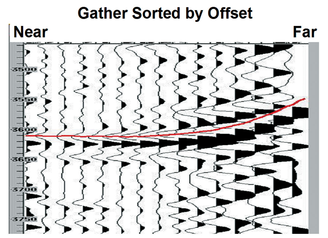
To explore for fractures we need to identify changes in the earth related to Horizontal Transverse Isotropy or HTI – these are the velocity variations that occur as a function of azimuth. Most seismic processing is readily able to handle Vertical Transverse Isotropy (VTI) also known as Layered or Polar Anisotropy. VTI appears on NMO corrected unmigrated gathers and pre-stack migrated gathers as the well known ‘hockey stick’ at the far offsets or high incidence angles (Figure 2). The velocity used to move-out or image the gather was generally correct for the near offsets but not the far so the event isn’t flat. The seismic processor can correct this effect post migration or include VTI in the migration to properly image the event. VTI, if present, must be addressed before we can search for HTI anomalies (Figure 3).

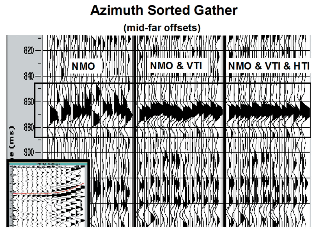
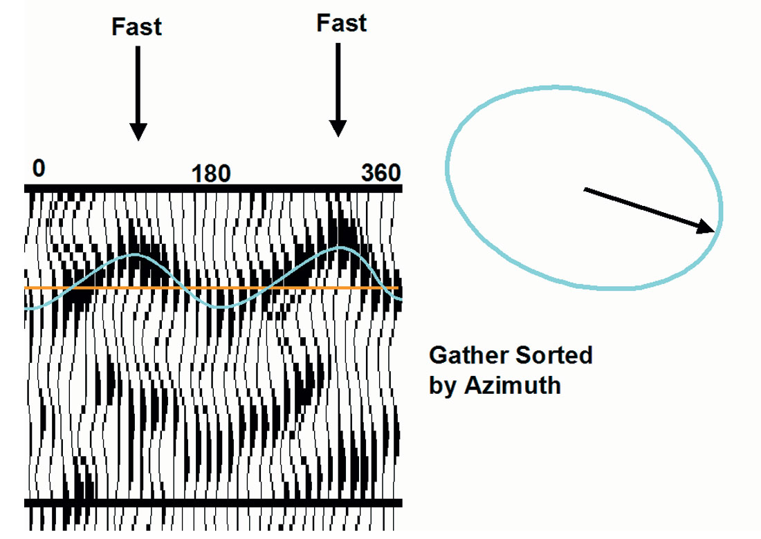
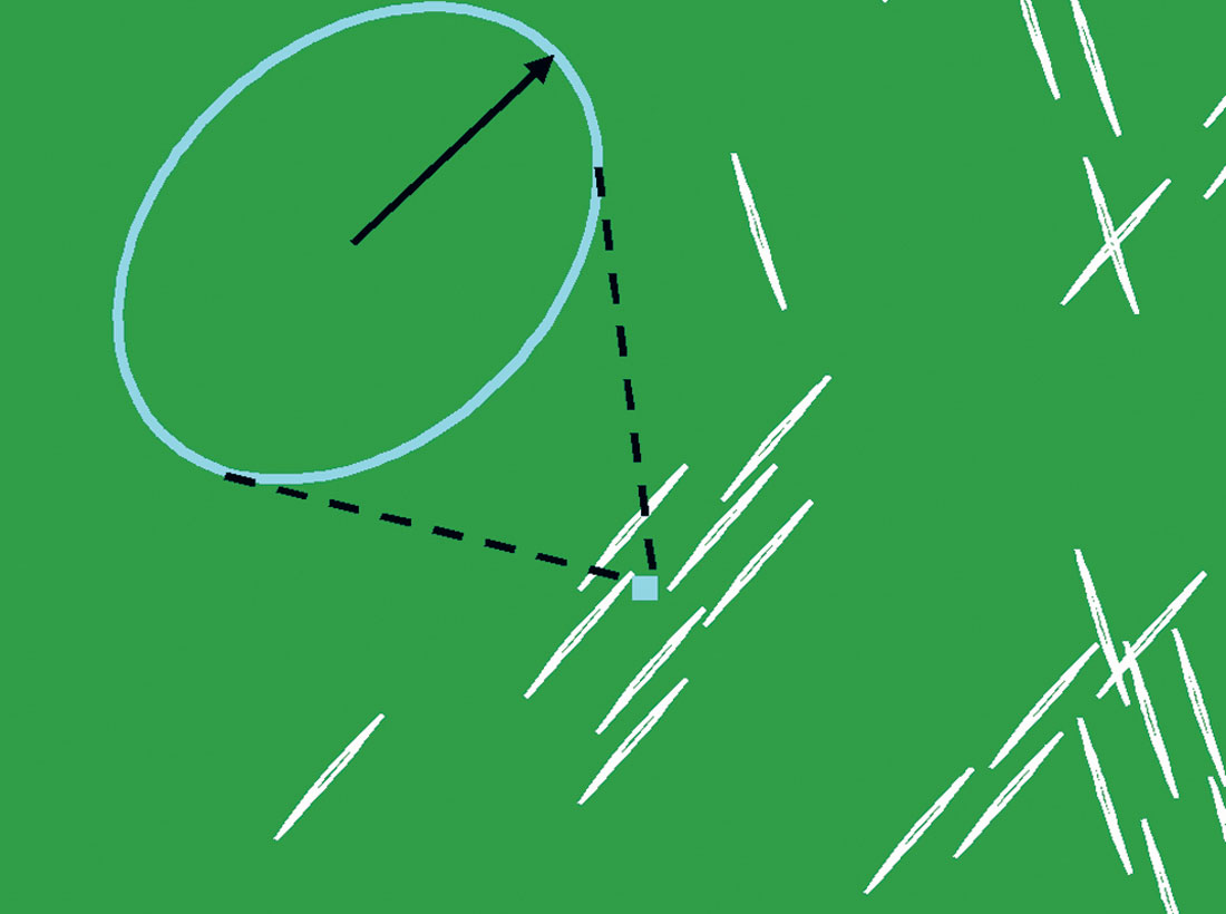
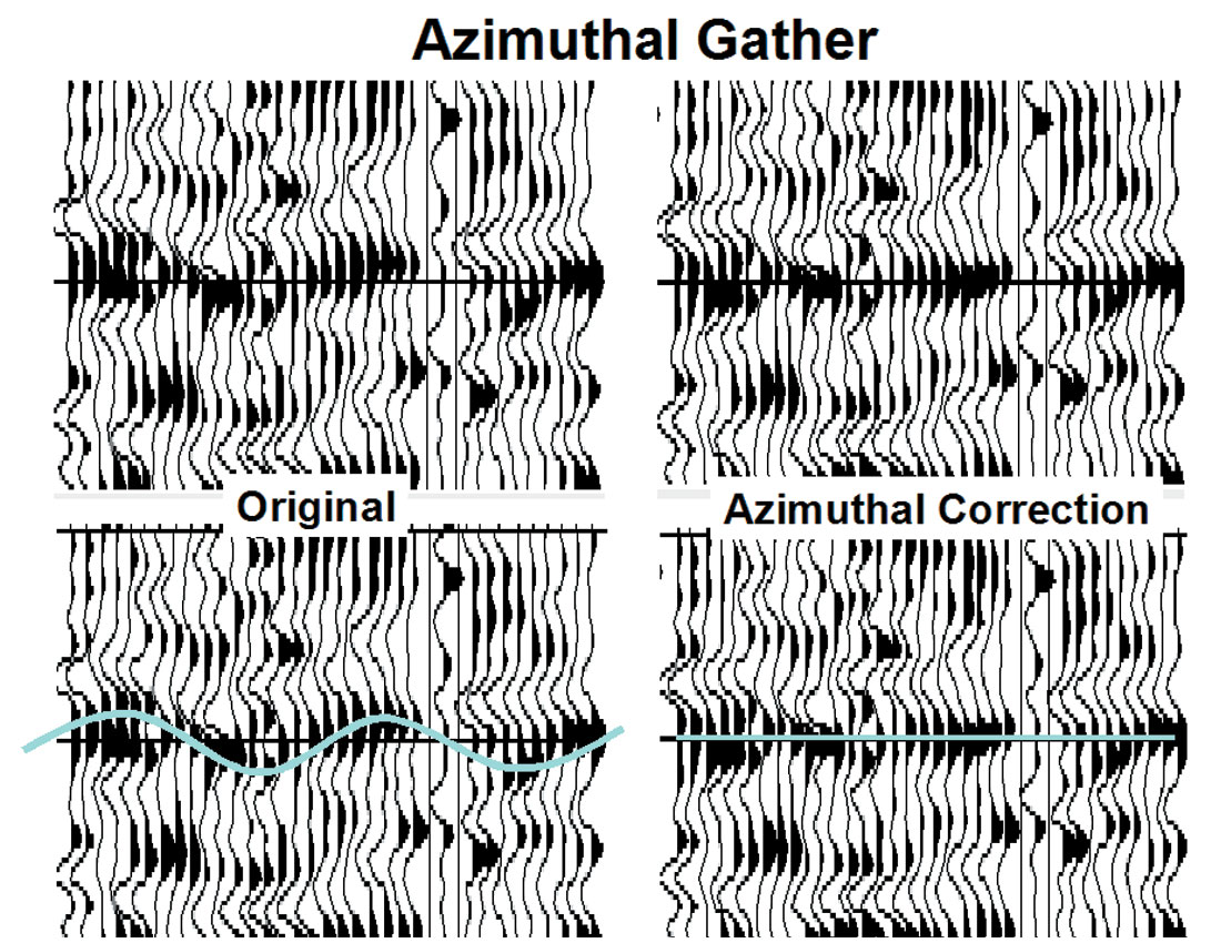
Identifying HTI velocity anomalies is the initial goal of most azimuthal velocity analysis. Open fractures can cause changes in the seismic velocity field that vary with azimuth. At vertical incidence there is no effect, but at higher incident angles the compressional wave can be delayed passing across a vertical fracture set. Parallel to the fracture set there is no slow-down. In areas of open conjugate fracture sets the velocity is slowed down in multiple directions and neither multicomponent nor azimuthal techniques will effectively predict the open fractures. These areas are best detected by looking for relatively low interval velocities computed from the isotropic velocity field. Azimuthal analysis works best where there’s a dominant stress field opening a fracture set in one direction while closing the other sets. This creates the sinusoid pattern apparent in Figure 3 (sorted by azimuth and not offset). In an isotropic world the NMO corrected event shown would be flat. The periodic late and early arrivals indicate slow and fast directions – an azimuthal velocity anomaly (Figure 4). The sinusoid can be represented by an ellipse with the long axis describing the fast direction and the degree of ellipticity describing the difference between fast and slow velocity.

Azimuthal Analysis

Azimuthal analysis that targets fracture prediction attempts to identify the sinusoids/ellipses across a 3D volume and determine the magnitude of the anomaly and its orientation or azimuth. Typical azimuthal velocity anomalies are a 1-5 % change in the background RMS velocity field but can reflect interval velocity differences of 5-30% (fast velocity versus slow velocity). Identifying areas within a reservoir interval that exhibit azimuthal velocity variations requires removal of overburden azimuthal effects to properly extract the interval velocity anomalies and map the fracture swarms (Figure 5).

With an expectation that fractures or stress field variations exist within a target reservoir section we proceed with the analysis of the 3D dataset. The first critical issue is the seismic acquisition. Does the acquisition sample the azimuths sufficiently for the results to have meaning. Sampling requirements depend on the kind of azimuthal analysis being performed but all techniques benefit from rich azimuth sampling. Optimal acquisition contains relatively uniform coverage at the target for all azimuths in incident angle ranges between 20-40 degrees. Marine cable surveys are typically under-sampled for azimuthal processing but most modern land 3D surveys have enough information to search for azimuthal anomalies.

Finding Sinusoids

Historically the process of finding the sinusoids that indicate an azimuthal velocity anomaly has been performed in unmigrated super-gathers (gathers created by summing approximately nine gathers into a single bin and sorting by azimuth). More recent techniques have attempted to use various workflows to bring the process into migrated space. Below is a summary of current techniques and the sequence of steps performed to find the velocity anomalies and compute the final migrated stack (AAD = Azimuthal Anomaly Detection).

1. Unmigrated Super-binned Gathers, AAD – Azimuthal NMO (RNMO by azimuth) – Isotropic PSTM and Stack
2. Sectored Techniques
   1. Sectored Gathers – Isotropic Migration of Sectors – AAD, RNMO, Stack
   2. Isotropic Migration into Azimuth and Offset sectors – AAD, RNMO, Stack
3. Azimuthal Migration Velocity Analysis, AAD, Azimuthal Migration, Stack

The super-gather approach (1) provides higher fold for the sinusoid search at the expense of some lateral resolution. The downside of this approach is that working in unmigrated space means that subtle fracture anomalies are smeared across the fresnel zone at the target, signal-to-noise is poor and a flat world must be assumed (the actual location of the anomaly may move updip in migrated space). Attempts to move the search into migrated space have generally involved some form of sectoring - either dividing the input to migration into azimuth sectors (2a) or telling an isotropic migration what azimuth each input trace represents and preserving that information on output (2b). The resulting imaged gather contains both offset and azimuth information forming a mini 3D (cross-spread gathers). The imaged gather volumes are scanned for residual NMO that fit a sinusoid. Lynn (2007) compared an unmigrated super-bin approach with an input sectored migration approach and found the migrated results less reliable for a Barnett shale project. The sectored migration provided just four values per 180 degrees of azimuth leaving considerable uncertainty in finding the correct sinusoid. While the migration addresses dip, the assignment of azimuth values to output sectors assumes a surface geometry from the acquisition that assumes a flat world.

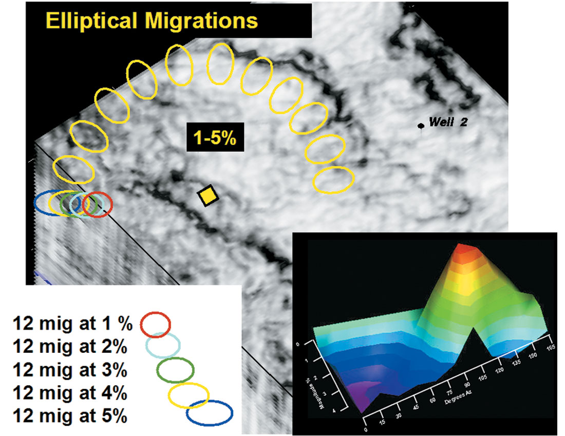
The third technique for finding the sinusoids involves allowing the migration to identify the fast and slow axes using all azimuths (no sectoring). After addressing VTI (if present) a time window covering the zone of interest is migrated using a series of migration operators that vary the amplitude of the sinusoid and the azimuth of the fast direction. Small changes in the operators create a semblance-like look at the best fit sinusoid in image space (Figure 6). The process typically involves imaging a portion of the dataset 60-120 times to identify the fast direction and the magnitude of azimuthal velocity variation. The impulse response of the migration operator is an ellipse effectively testing a series of sinusoids to see what works best to focus the events at a target location. The azimuthal migration velocity analysis suffers less from lower azimuthal sampling by the acquisition (compared with the super-gather and sectored approaches) and resolves smaller azimuth changes – outputting a minimum of 12 azimuths for each azimuthal velocity magnitude tested.

Imaging

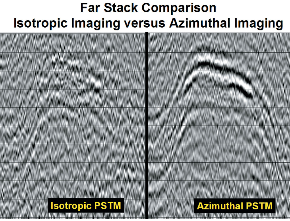
In the presence of azimuthal velocity variations an isotropic migration can misposition events, destroying the mid to far offsets and degrading the stacked image. In areas of strong azimuthal velocity variations, single azimuth shooting (2D data) may outperform 3D imaging if azimuthal variations aren’t addressed in the 3D. In the past, typical imaging flows designed to address HTI anomalies have involved either basic trim statics followed by an isotropic PSTM or Azimuthal NMO followed by PSTM. Including the azimuthal parameters in the final migration can recover an image that standard time and depth imaging techniques fail to focus (Figure 7).

Azimuthal Interpretation

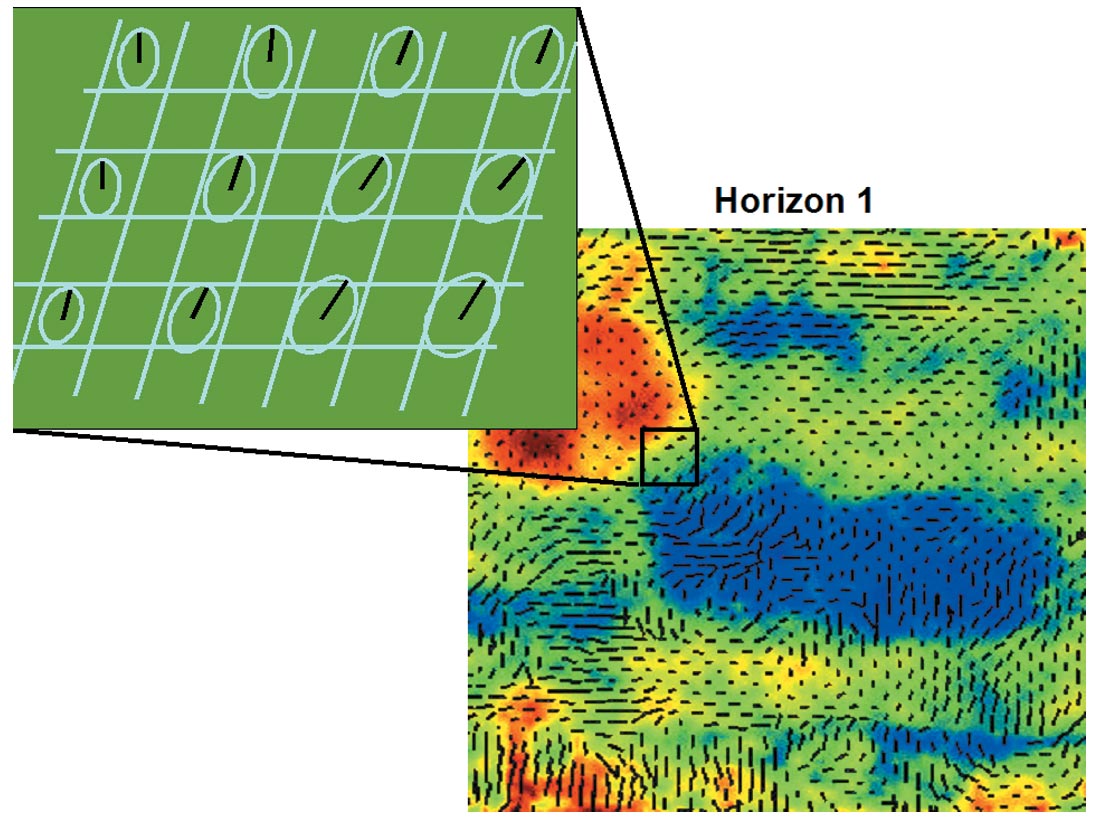
With the azimuthal properties extracted from the above migration analysis two volumes are created that describe the detection of sinusoids – an interval velocity factor volume and an azimuth volume (Figure 8). The factor volume represents the percent change in interval velocity from the background isotropic velocity field. Low factors mean there were little or no azimuthal variations detected for that interval. High factors imply a large azimuthal variation but need to be confirmed by looking at the gathers. Azimuthal analysis is a form of pre-stack analysis (like AVO – Amplitude Versus Offset) so false anomalies will occur due to noise or poor azimuthal sampling. Looking at the gathers is the minimal test for determining the validity of an anomaly (Figure 9).

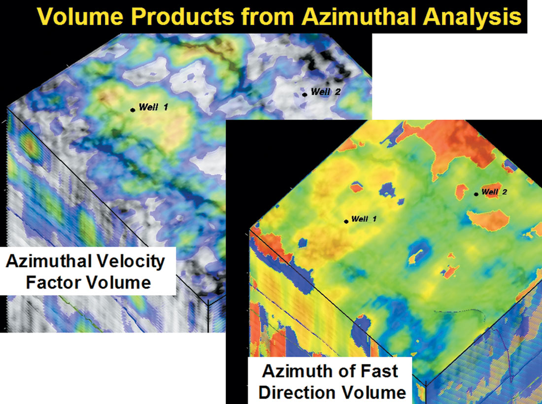
The azimuth volume represents the direction of the fast velocity. In areas of minimal azimuthal velocity variations the azimuth volume is unreliable (there is no fast direction) so interpreting an azimuth volume must be done in conjunction with the factor volume. Two workflows are common for comparing and interpreting the pair of attributes. The first involves combining the two values to make a vector indicating azimuth and magnitude of the velocity anomaly (typically at a specified horizon) (Figure 10). Beneath the vector one can post the background velocity or some quality factor from the sinusoid fit. The second involves either co-rendering or dual displaying both volumes extracted at the target horizon and interactively comparing one to the other.

Azimuthal AVO

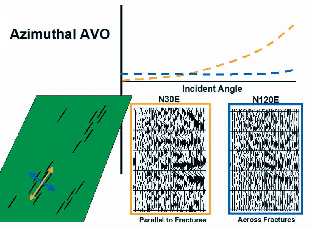
Once the velocity changes and azimuths for a particular 3D volume are determined, one can investigate the fracture potential further by comparing the AVO responses for a target as a function of azimuth (Ruger, 1998, Sen 2007) (Figure 11). AVO by azimuth (AVOA) can be performed in unmigrated super-bin space (Luo, 2004) or post migration. Migrated AVOA requires sectoring the output of the migration into different azimuth bins that can be compared with a sectored NI stack or Near Trace stack to help identify azimuthal AVO anomalies. As discussed earlier, sectoring requires greater azimuthal sampling in the input dataset to provide a reliable Azimuthal AVO solution. Typical AVOA workflows involve performing an isotropic PSTM into azimuth and offset bins, addressing residual NMO associated with azimuthal velocity variations followed by some type of AVO analysis on each of the azimuth groups. Correcting for the azimuthal velocity variations in the migration replaces the above residual NMO step and should provide a more focused cross-spread gather for the AVOA analysis.

Conclusions

Fracture prospecting is a critical component of field development in most hard-rock settings. P-wave seismic data offers the potential to identify and map fracture swarms using azimuthal velocity analysis and azimuthal AVO. Full azimuth azimuthal imaging avoids the pitfalls of under-sampled azimuthal sectoring approaches and can deliver azimuthal anomaly maps indicative of open fractures. Inclusion of azimuthal velocity variations in the imaging offers better event positioning for more sharply focused stacks. Sectoring for Azimuthal AVO benefits from a migration that recognizes azimuthal velocity variations in the migration instead of addressing the problem in a residual NMO analysis.