AVO and the General Inverse Theory

Introduction

The 1980s saw the development of two new technologies: AVO and general inverse theory. In those days, general inverse theory was applied to full waveform inversion, compared to which AVO is a very simple problem. Almost two decades later we observe that the interest for full waveform inversion has waned, probably because the problem was deemed too complex, while the interest for AVO is alive and well. The purpose of this paper is to use the simple example of AVO, and the lessons learnt for more than 15 years, to better understand the intricacies of general inverse theory.

General Inverse Theory

Consider a linear relationship G between some data d and model parameters m:

The data are made of N records and the model contains L unknown parameters. G is therefore a N x L matrix. I only consider the case when there are more data than unknowns, therefore N is larger than L. The first step in the least-squares inversion process is to compute the normal equations. They are given by:

Assuming the data are made of independent records of equal uncertainty (or accuracy), the expression for the least-squares estimation of mˆ is:

where C_m is the a priori model covariance matrix. It represents the starting hypotheses on the model parameters. Its main goal is to stabilize the inversion process and make sure the inverse matrix does not explode. It is often chosen as a constant diagonal matrix, in which case it is referred to as the damping matrix (or “prewhitening” for deconvolution). In the least-squares theory, the a posteriori model covariance matrix represents the uncertainties of the estimated parameters. It is expressed as:

The value of this a posteriori covariance matrix has often been overlooked. Yet it is in my opinion the most important piece of information delivered by the least-squares theory. The diagonal terms represent the uncertainties of all estimated parameters (the square of the standard deviation), and the off-diagonal terms represent the statistical correlations between the various parameters. Equation (4) also expresses the relative importance of the original physical relationship and the a priori covariance matrix. If the latter overwhelms the former - meaning we either distrust the data or equation (1) - the resulting uncertainties are identical to the original uncertainties. In other words, the inversion process has not brought anything to what was already known (or assumed). Conversely, when the a priori covariance matrix is small enough to be neglected, the uncertainties are purely a function of equation (1). This can be dangerous if the problem is ill conditioned, because noise will be blown up. It is then almost an art form to find the right level of damping. The best-known illustration is the deconvolution problem: The damping level must be such that the frequencies dominated by noise are not boosted. Yet the side effects of pre-whitening, especially on phase, are far from negligible (see for example Gibson and Larner, 1984). Next, we will see what the a posteriori covariance matrix means for AVO inversion.

AVO Inversion

For the AVO problem the data are made of pre-stack reflection coefficients and the model parameters are made of two (sometimes three) attributes. For this paper, the intercept A and the gradient B will be considered. We have:

The normal equations can be written as:

The first equation actually shows that the stack S is a reflectivity series at a certain angle of incidence. The second equation defines another term F, itself a reflectivity series at an incidence angle. I will come back to this term later. For the AVO problem, the linear system can be solved without the use of damping. Hence, the least-squares solution is:

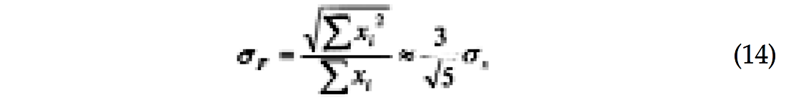
where σ_x is the standard deviation of the sine-squared series:

It is straightforward to extract the a posteriori covariance matrix from equation (7). The uncertainties for intercept and gradient are:

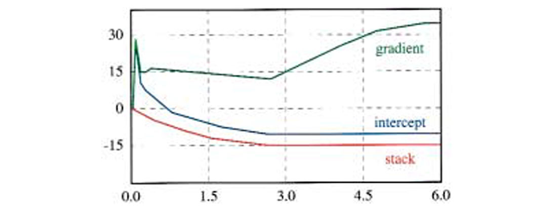
where σ_s is the stack standard deviation. Figure 1 shows how these uncertainties behave for a typical marine geometry. The stack uncertainty decreases with the square root of the fold and reaches a plateau (-15 dB) associated with maximum fold (30) below the mute zone. Intercept and gradient need at least two-fold to be computed, which explains why their uncertainties are so high for shallow times. The intercept decreases as the fold builds up, and eventually reaches a plateau above the stack level. The gradient on the other hand first reaches a plateau within the mute zone and then steadily increases. The plateau is associated with the mute function, which roughly follows a constant incidence angle (30 degrees in this case). The slight decrease corresponds to fold building within the mute zone. To understand these behaviors consider the following approximation, only valid for a limited range of incidence angles:

Plugging equation (10) into equations (8) and (9), and retaining only the highest power of N leads to:

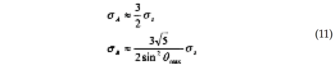
The first expression shows that the intercept uncertainty plateaus 3.5 dB above the stack level. The gradient uncertainty is inversely proportional to the square of the maximum incidence angle, which explains why it increases so much below the mute zone.

The a posteriori covariance matrix does have off-diagonal terms, which means that intercept and gradients are statistically correlated. The correlation coefficient is given by the off-diagonal term divided by the standard deviations:

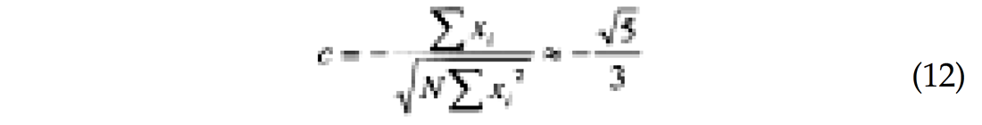
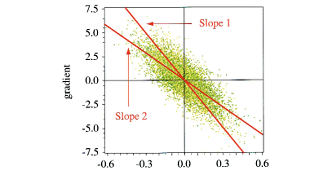
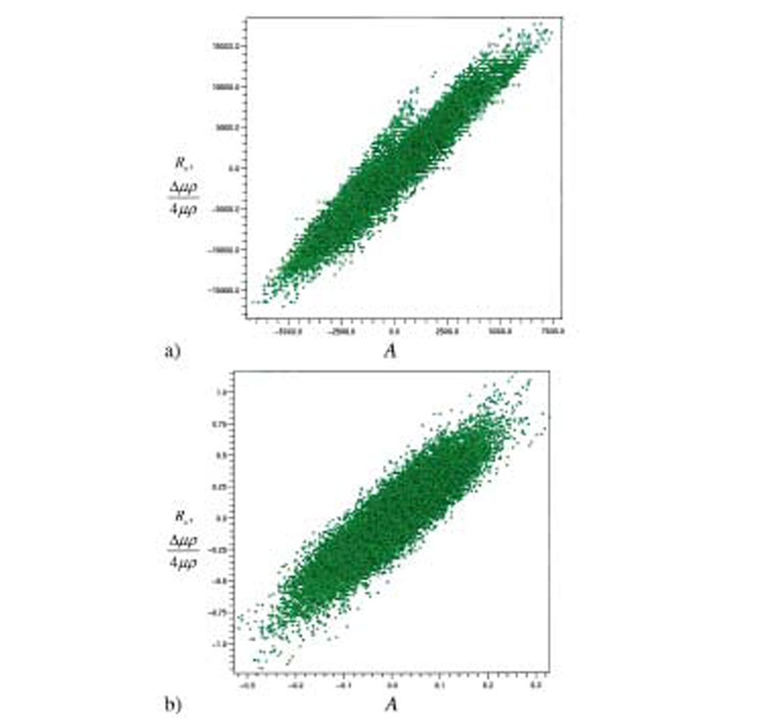
The small angle approximation gives a negative correlation in the order of -0.75, which is fairly high. Figure 2 shows a crossplot of intercept and gradient computed on pure random noise. As expected, there is a difference of scale (the gradient is boosted due to the larger standard deviation) and a negative correlation. This correlation is particularly unfortunate because it coincides with the trend expected from brine-filled shales and sands (Castagna and Swan, 1997).

Attribute Correlation

Equation (12) establishes the existence of a statistical correlation between intercept and gradient. This correlation is actually given by equation (6). It is easy to show that stack and gradient are statistically uncorrelated, as well as intercept and F. This is not by chance; this is a general result of the least-squares theory. Equation (6) describes two linear relationships between intercept and gradient. The first one relates the intercept to the two independent variables stack and gradient. It corresponds to Slope 1 in Figure 2. Similarly, the second equation relates the gradient to the two independent variables intercept and F, and corresponds to Slope 2. A linear regression on the scattered points in Figure 2 would lead to either slope depending on axis orientation. Computing intercept as a function of gradient yields Slope 1 while computing gradient as a function of intercept yields Slope 2. These two slopes are not inverse to each other, but their product is equal to the square of the correlation coefficient in equation (12), as predicted by the general least-squares theory. (The slopes can only be inverse to each other when the correlation coefficient is ±1, which means that all samples are perfectly aligned.)

Crossplotting intercept and gradient is often used for AVO analysis. The points that stand out of the background trend generally correspond to hydrocarbon bearing sands. Thus, one of the best hydrocarbon indicator is the fluid factor which measures the distance of any crossplotted point to the fluid line (the background trend). This attribute is generally obtained statistically (see for example Fatti et al., 1994). The background trend is removed by combining intercept and gradient in a linear way, the linear relationship being derived by regression analysis on the crossplot. If the background trend is due to noise (like in Figure 2) the fluid factor is either the stack or F - depending on axis orientation, intercept as a function of gradient or the opposite.

As expressed in equation (6), F is the reflectivity at angle Ω with:

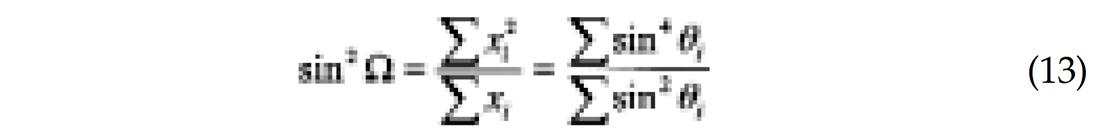
Under the small angle approximation, Ω is about 80% of the maximum incidence angle. Thus, F can be assimilated to the maximum angle stack. As such, it is a decent hydrocarbon indicator, and actually a much better indicator than the stack. Therefore, if the background trend is due to noise, the fluid factor is at best a far angle stack.

In addition, F is a very reliable attribute with a standard deviation:

which is actually better than for the intercept.

There are many other AVO attributes, but they are all linearly related to intercept and gradient. Because these two are correlated (non-orthogonal), they do not represent the best basis. Instead, I choose to use as reference A and F. They represent respectively the reflectivity series at angle 0 and Ω, and they are orthogonal. Standard AVO attributes can then be expressed as:

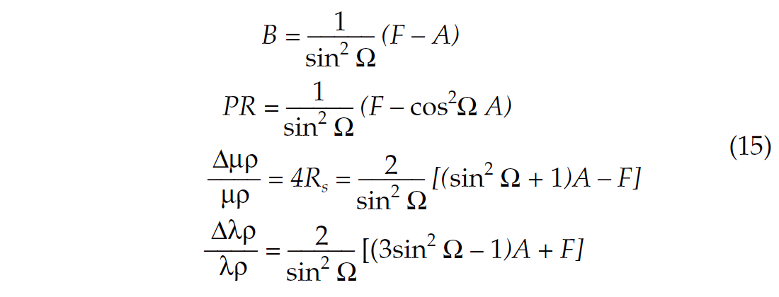
where PR is Verm and Hilterman’s Poisson’s reflectivity (1995), R_s is shear-reflectivity and λ, μ and ρ are Lamé parameter (Goodway et al., 1997). Note that when Ω is close to 35 degrees, the λρ reflectivity is equal to 6F and is therefore uncorrelated with the intercept.

Equations (7) and (15) contain identical information. Yet equation (15) is a lot more telling. First, it gives immediate indication of attribute reliability. Assuming Ω is close to 30 degrees, we see the gradient is the difference between A and F multiplied by 4. Any amount of noise in the data will therefore be boosted in the process, as illustrated in Figure 1. Second, statistical correlations between the various attributes are readily available from equation (15).

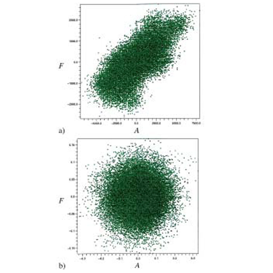
In their paper, Fatti et al. compute the fluid factor by linear combination of intercept and shear-reflectivity. Equation (15) shows that in the presence of noise, the resulting fluid factor is F. Figure 3 illustrates the issue with real data from the Blackfoot survey: The trend observed in the A - R_s crossplot is very similar to the noise crossplot. Therefore, the fluid factor computed according to Fatti et al. for these data will result in F. Instead, the A - F crossplot, which also shows a trend but with a much weaker correlation, is meaningful because there is no expected noise trend (Figure 4).

Other Inversion Schemes

The first reaction when observing the unreliability of the gradient is to use some sort of damping. Damping is efficient at reducing the scale of the gradient, but it does not remove the statistical correlation (Herrmann and Cambois, 2000). Hence, it can be misleading by providing a false sense of confidence in the gradient while still resulting in a biased fluid factor.

Another approach to inversion is singular value decomposition (SVD). This method decomposes the data and model in orthogonal bases (eigenvectors), which makes the inversion a diagonal problem. In a way it is very similar to the approach described above with the uncorrelated attributes, except that in SVD the eigenvectors generally do not have physical meaning. Eigenvectors actually make sense for specific problems, such as deconvolution where they roughly represent sinusoids of varying frequencies, and surface- consistent decomposition where they represent spatial wavelengths (Wiggins et al., 1976). Since the eigenvectors are generally meaningless (as referred to AVO inversion), the inverted data are transformed back into the model basis. Thus, the orthogonal nature of the SVD approach is not utilized and the statistical correlations are re-introduced.

Conclusions

The two-term AVO problem is probably the simplest inverse problem one could think of. Yet the issues it raises are far from trivial. In particular, the matrix to be inverted is ill conditioned and the presence of off-diagonal terms guarantees attribute correlation. This correlation, when ignored, can lead to biased results, particularly when crossplotting is involved. Damping, the usual cure, resolves the conditioning problem but does nothing against statistical correlation, which can be even more misleading.

An alternative approach identifies meaningful uncorrelated attributes, which can be used to compute all other attributes. This approach readily provides an estimate of uncertainties and correlation of the various attributes. Although this paper has only shown applications to the AVO problem, the concepts can be extended to any inverse problem. The underlying principle is that instead of spending huge amounts of computer time inverting oversize matrices, it is much more valuable to study which attributes are uncorrelated and use them to directly solve the problem. The inversion will be a lot faster (diagonal) and the artifacts will be immediately understood.