Applications of DC Resistivity and Magnetotelluric Methods in Exploration

The Schlumberger brothers were the first to use the direct current (DC) resistivity method for exploration in oil well boreholes in Russia during the 1920’s. A unique phenomenon, now referred to as induced polarization (IP) chargeability, was noticed at the time, but not understood until simultaneous developments in both Russia and North America in the 1950’s. This lead to the development of the time domain and frequency domain IP methods. Combined DCIP surveys have become mainstays in mineral exploration, with the two measurements (resistivity and chargeability) both being recorded at the same time using the same equipment. DCIP was briefly used in the late 1970’s and early 1980’s for hydrocarbon exploration using very large truck-mounted generator/transmitter combinations and large receiver dipoles, but with limited success (Seigel et al, 2007).

DCIP recording systems went through a significant advance when digital distributed array technologies developed for seismic were adopted. In addition to facilitating large scale, high resolution DCIP surveys in both 2D and 3D, these new systems opened the door to passively recording naturally occurring EM signals, a method called magnetotellurics (MT).

MT is a natural-source electromagnetic (EM) method. The mathematical groundwork was developed virtually simultaneously in Russia, Japan and France by Tikhonov, Rikitake and Cagniard respectively (Chave and Jones, 2012). Commercial use of MT occurred in the late 1950’s in the USA, primarily for geothermal exploration (reservoir sealing, high-conductivity, impermeable clay layers at depth); in Russia in the 1970’s for hydrocarbon exploration (wildcat exploration in difficult terrain), and in North American and African mineral exploration (initially for diamonds to define the base of the craton, now routinely for defining mineralizing systems from surface to depth).

Modern recording systems such as Quantec’s TITAN 24 (2D) and ORION 3D routinely record DCIP and MT all in one survey. Typically, the DCIP is recorded during the day as active crew involvement is required to perform current injections, and the MT is recorded passively during the night when the naturally occurring signals are the strongest. DCIP can provide a relatively high-resolution model to a depth of around 700 m, with the MT model starting at approximately 500 m depth and extending down to several km, with depth being dependent on acquisition geometry.

This article will focus on the MT method, but as MT data are often recorded along with DCIP data, the latter will be mentioned in case study results when relevant.

Fundamentals of the MT Method

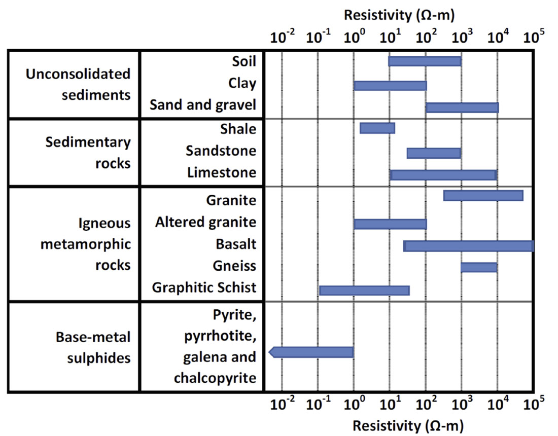
Resistivity in rocks is a measure of the relative ability of a rock volume to transmit an electrical current. The flow of current through a rock is a function of one or more of the following:

• Electrolytic conduction – ionic movement in pore and fracture-filling fluids,
• Cation exchange – a common occurrence in many clay mineral assemblages,
• Electronic (ohmic) conduction in graphite and metallic sulphides, and
• Dielectric conduction – where an alternating electric field causes ions in a crystalline structure to shift cyclically.

As a result, the resistivity of rocks and minerals is highly variable and further complicated by the fact that most rock forming minerals are insulators. In most instances, current flows via ions in pore fluids (i.e. electrolytic current flow) and hence a major control on resistivity is porosity. The measurement of resistivity, particularly in a borehole, is often used as a proxy for porosity and density. Additional factors associated with porosity include the degree of fluid saturation in the rock and the nature of the fluid (i.e. the concentration of dissolved salts in the fluid). Native metals and graphite pass current by electron motion (i.e. electronic current flow), the efficiency of the current flow determined by the crystal habit of the constituent minerals (i.e. platy or not). Typical resistivity ranges for various minerals and rock types are illustrated by Figure 1.

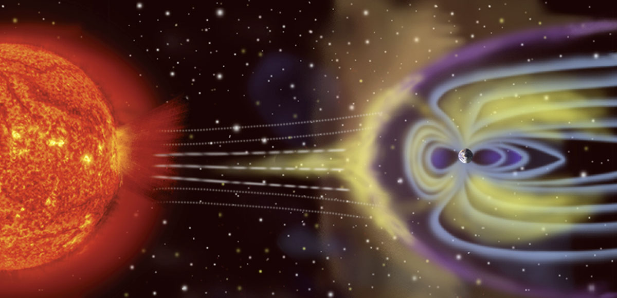
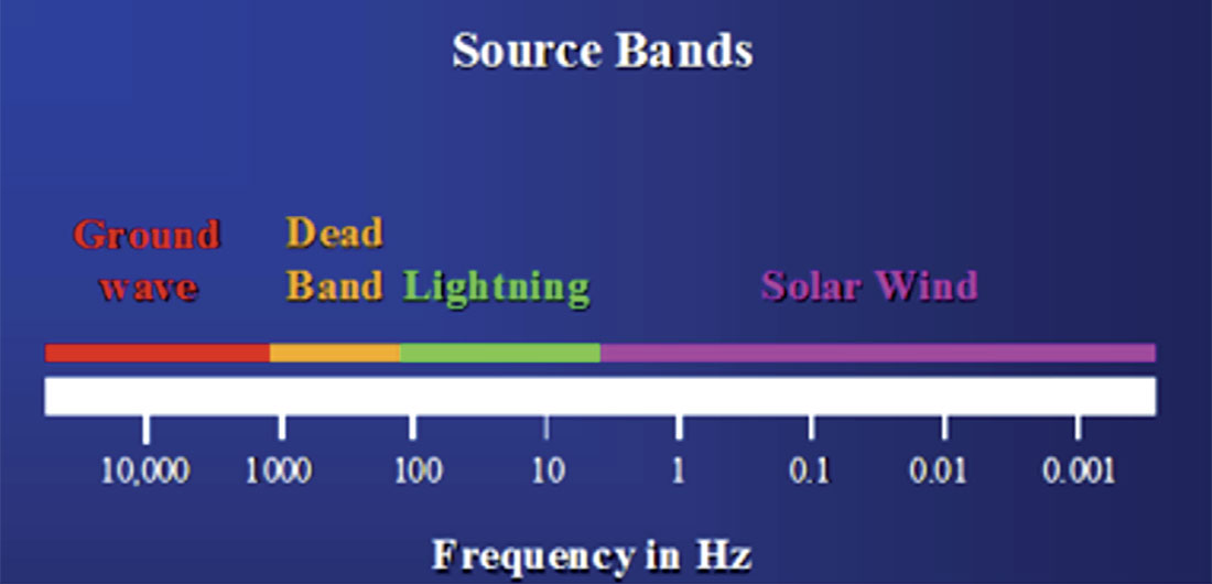
The MT method depends on naturally occurring electromagnetic waves as its source. These are generated in the earth’s atmosphere by a range of physical mechanisms, and their decay rate within the earth is dependent upon their wavelength. In general, high frequency signals originate from lightning activity, intermediate frequency signals are the result of ionospheric resonances, and low frequency signals are generated by sun spot activity (Figure 2). Figure 3 illustrates the electromagnetic frequency range for MT. There is a frequency band for which no natural source energy is typically present, and this is referred to as the “Dead Band”. A complete review of the method is presented in Vozoff (1972) and Orange (1989).

By measuring the broadband frequency content of the natural electromagnetic field, it is possible to construct a model of the resistivity structure of the earth from the near surface to great depths. Figure 4 illustrates this frequency-dependent concept referred to as skin depth.

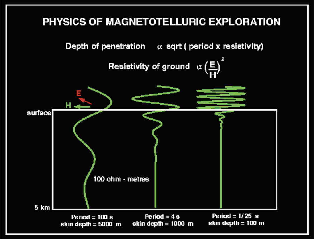
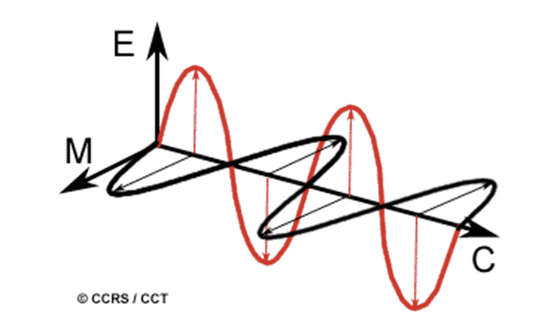
The natural EM waves travel through the rock and are recorded at stations deployed on the surface, specifically their electric field (E) and magnetic field (H) components (Figure 5). The relationship between the parameters of the electric E-field signal (i.e. the voltages over Ex and Ey dipoles), the magnetic M-field signal (i.e. the emf’s registered on Hx, Hy, and Hz inductive coils), ground resistivity (i.e. ρ) and frequency, is described by the Cagniard Resistivity Relation (Cagniard (1953)).

The measured MT impedance Z, defined by the ratio between the E and H fields, is a tensor of complex numbers. This tensor is generally represented by its two off-diagonal elements. In a 1D earth model where resistivity varies only with depth, there is no strike direction and the two off-diagonal impedances are equal. In the 2D case, where resistivity varies with depth and perpendicularly to the strike, and when the profile is set perpendicular to the strike direction, the two off-diagonal elements are not equal but reflect the variation of the resistivity along two directions, one parallel and the other perpendicular to the strike, i.e., the TE (Transverse Electric; E parallel to the strike) and the TM (Transverse Magnetic; E perpendicular to the strike) modes. The impedance phase data range between 0 radians and ϖ/2 radians. A phase value of ϖ/4 radians represents a homogenous earth case. Lower phase values occur at frequencies where the data transition through a conductor-over-resistor interface; higher values occur where the data transition through a resistor-over-conductor interface.

Both TE and TM impedances are represented by an apparent resistivity (a parameter proportional to the modulus of Z) and a phase (argument of Z). The variation of those parameters with frequency relates the variations of the resistivity with depth. The high frequencies sample the shallow sub-surface and the low frequencies the deeper parts of the Earth. However, the apparent resistivity and the phase have an opposite behaviour. An increase of the phase indicates a more conductive zone than the host rocks and is associated with a decrease of the apparent resistivity. The objective of MT data inversion is to compute a subsurface resisitivity distribution that explains the variations of the MT parameters, i.e. the response of the model that fits the observed data. The solution however is not unique and different inversions must be performed (different programs, different conditions) to gain confidence in possible target anomalies and eliminate possible artefacts.

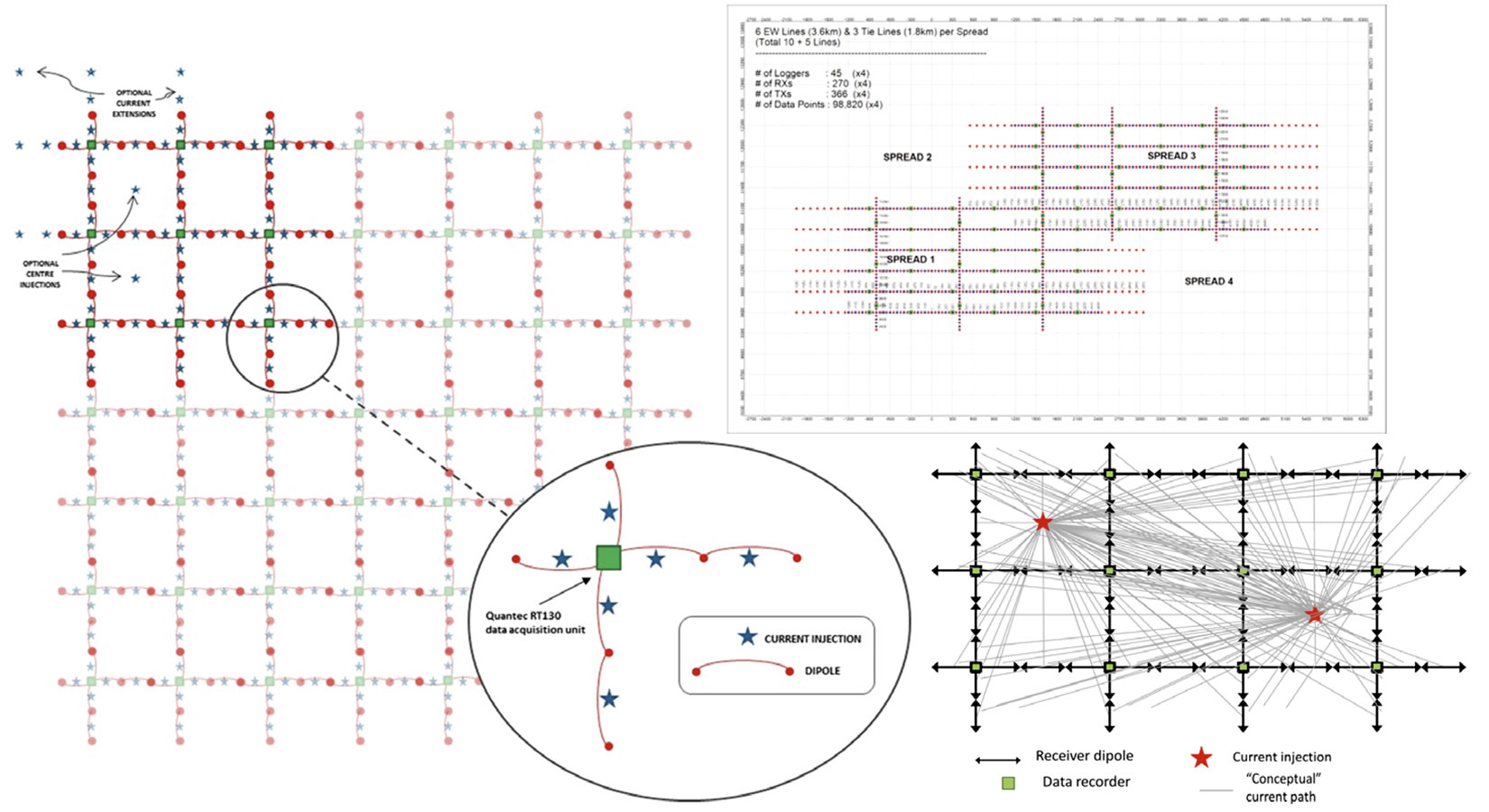
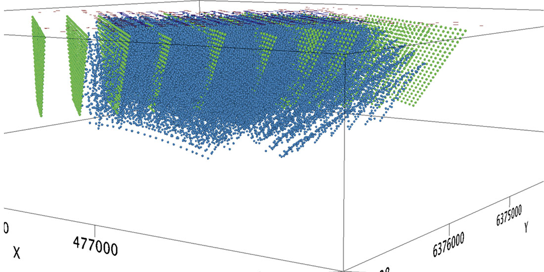
The depth of investigation is determined primarily by the frequency content of the measurement and the conductivity of the Earth. The investigation depth from any individual sounding may easily exceed several tens of kilometres. However, the data may only be confidently interpreted when the aperture of the survey array is comparable to the depth of investigation. To accurately capture the lower frequencies associated with greater depth, long recording times of many hours are required. Inversion of MT data is mathematically complex and computationally expensive. Advances in computing power in recent years have made 3D inversion possible. The benefits of 3D DCIP acquisition over 2D are analogous to the differences between 2D and 3D seismic. The advancement from 2D DCIP to 3D DCIP acquisition and inversion has extended the depth of investigation and improved the localization of anomalies, mainly due to a minimum 10-fold increase in data coverage (Figure 6), and the ability to record a full and balanced range of azimuths. Figure 7 illustrates the hypothetical difference in coverage for a 2D survey (green dots) and a 3D survey (blue dots).

Results

Selected MT survey results are presented in this section.

Porphyry

A typical application of 3D DCIP and MT has been in the exploration and definition of porphyry systems in mineral exploration. The following example is from an exploration program completed at high altitude (from 3800 to 4550 m ASL) in the Chilean cordillera over the Santa Cecilia porphyry target of the Cerro Grande Mining Corporation. The exploration objectives for the DCIP + MT survey were to follow up on previously completed MMI geochemical sampling, CSAMT (controlled source audio MT, i.e. high frequency active source MT) survey results, and drill results, to delineate near surface and deep-seated mineralization. More specifically, it was hoped the survey would provide models to:

• Map and delineate near-surface zones associated with Cu-Au-Ag mineralization and related alteration with the DC resistivity and Induced Polarization.
• Map and delineate deep-seated alteration zones that could control or host mineralization with MT.
• Focus drilling, thereby reducing overall drilling costs.

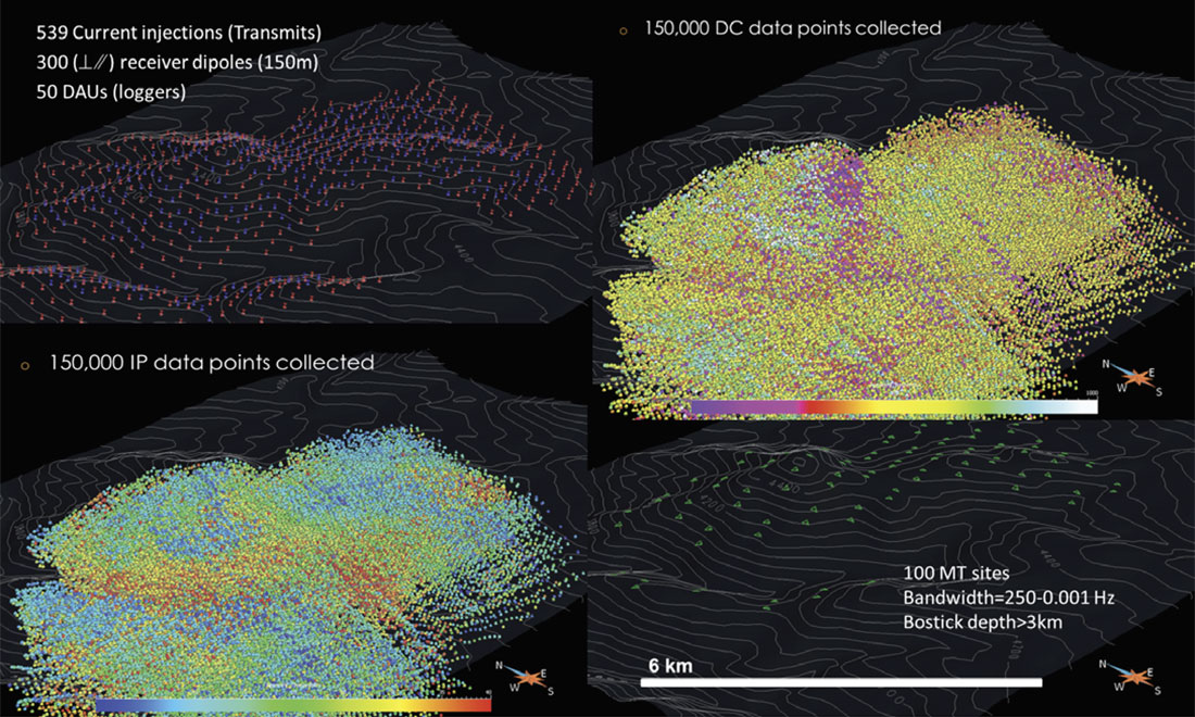
A total of 300 receiver dipoles each 150 m in length were deployed over an area of approximately 3 km by 6 km. A total of 539 current injections were completed to collect approximately 150,000 DCIP data points (Figure 8). At night the same equipment recorded the MT signal at 100 discrete (i.e. somewhat randomly located due to the difficult terrain) sites with a nominal station spacing of 450 m. The effective depth of investigation for an overnight read (4 to 14 hours of data acquired per site) was greater than 3 km. The data acquisition for the entire survey was completed in 16 days.

The DCIP data were inverted in 3D using licensed software developed by the University of British Columbia Geophysical Inversion Facility (UBC-GIF), and the MT data inverted using the 3D inversion software developed by Weerachai Siripunvaraporn and Gary Egbert (WSINV3DMT).

The survey was successful in mapping and delineating known alteration zones that host mineralization within the project area. The 3D inversion results provided a very detailed mapping and delineation of main areas of anomalous resistivity and chargeability occurring within the survey area and correlated very well with the limited near surface drilling results. By acquiring and inverting the data in 3D, fine ring structures consistent with mineralization in the near surface, and the overall extent, zonation and different geologic components of the porphyry system were mapped out (Figure 9).

Geothermal

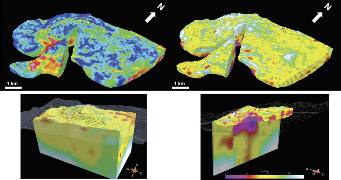
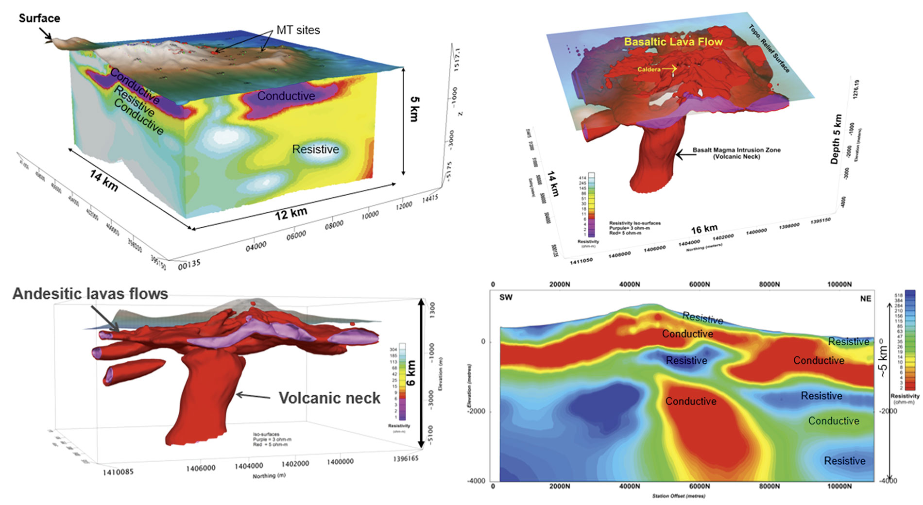
In a geothermal resource setting, usually only MT data is acquired since the near surface geology is of limited interest. In the following example from the southwestern USA, the MT method was applied to image the basaltic and andesitic lava flows associated with an active geothermal system, and the overall hydrogeological geothermal “plumbing” system. Approximately 200 discrete MT sites were deployed in a coarse grid pattern covering the 12 km by 14 km area of interest (Figure 10). The survey and subsequent 3D inversion of the MT data was successful in mapping the volcanic system and subsurface magma chambers responsible for the geothermal activity in the area.

A second geothermal example is from an area of south central Australia onshore of the Great Bight (Figure 11). Here, a large scale regional MT survey was undertaken in an attempt to identify hydrothermal resources.

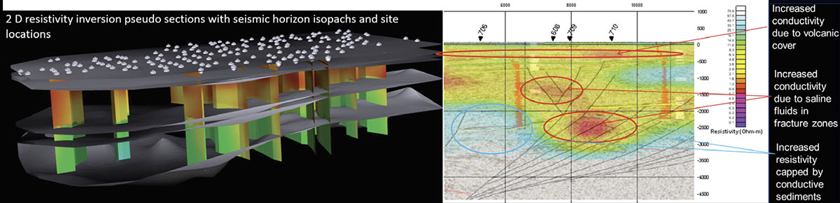
The area had previously been explored for oil and gas, and hence isopachs of the sedimentary formational contacts were available. A strong positive correlation was evident between the inverted MT model and some of the sedimentary contacts. There was also reasonably good correlation between the borehole conductivity logs and the inverted MT resistivity section. In parts of the survey area, the near surface cover rocks were of volcanic origin and of moderately higher conductivity (Figure 11). Within some of the faulted area, areas of increased conductivity due to saline fluids in fracture zones were identified. However, these fluid zones were not hot enough to be viable geothermal reservoirs.

Hydrocarbons

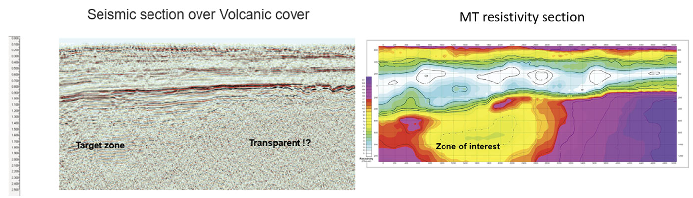
In the first example, from the Neuquen Basin in Argentina, shallow high acoustic impedance volcanics have prevented seismic surveys from effectively imaging the deeper hydrocarbon zones (Figure 12). An MT transect was completed, and the inverted data were integrated with the seismic. The volcanics, seen as an extremely high amplitude event in the seismic, were identified as a very conductive layer in the MT. Below that zones of moderate resistivity surrounded by high resistivities are potentially indicative of hydrocarbon zones, which are completely invisible to the seismic signal.

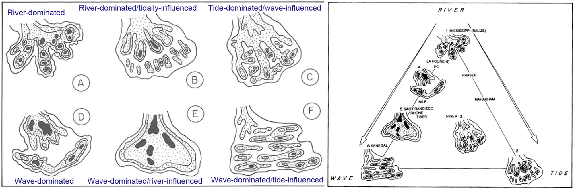
The second hydrocarbon example is from the edge of the Michigan Basin in southwestern Ontario. The hydrocarbon plays of the Silurian and Devonian along the edge of the Michigan Basin tend to be dominated by gas occurrences, often of small areal extent. The relatively shallow occurrence of these gas pools and the presence of existing infrastructure makes them relatively inexpensive to exploit. These plays are often encountered at depths ranging from surface seeps to over 1000 m depth. They are typically present as deltaic sands in paleo river channels and sandbars often classified as high wave energy, strong littoral drift models as defined by Coleman and Wright (1975) and Galloway (1975) (Figure 13). The implication, from a geophysical exploration perspective, is that the plays are complex, of small areal extent, and resemble the vein patterns seen in tree leaves. The reservoir rocks are therefore often narrow sandbars and river channels that may or may not be interconnected.

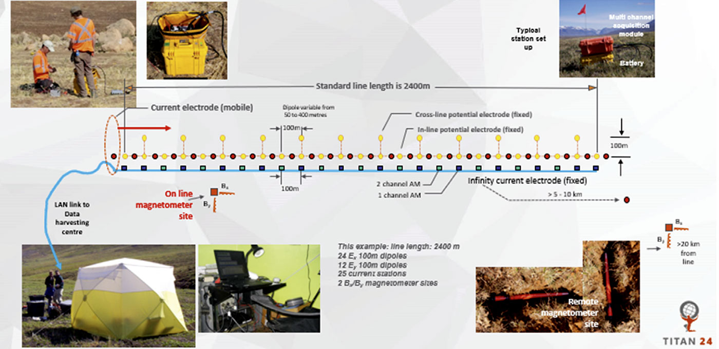
A TITAN 24 2D DCIP + MT survey was conducted as illustrated in Figure 14. An array length of 3600 m utilizing 150 m receiver dipoles was used. As would be expected, this general type of survey is very sensitive to spurious EM signals related to human activity. Southwestern Ontario is full of gas pipelines, high tension power lines, farm houses, telephone and power lines, etc., so care in locating the receiver dipoles and current transmit electrodes was required to reduce interference from cultural sources. During the data acquisition process, the time series being acquired at each receiver dipole was monitored to ensure that the best possible data was acquired. A transmit dipole of a=300 m was used for all current injections with the current dipole being “walked” through the distributed receiver array (effectively a DP-DP-DP array). As is typical, MT data acquisition occurred overnight using the receiver dipole arrays.

The near surface in this area is dominated by a thin (no thicker than 10 m), well-developed clay layer. The clays tend to be conductive and often present a problem for electrical and electromagnetic geophysical surveys, similar to the way shallow volcanics are a problem for seismic. In this example, the current injected into the subsurface was of sufficient amperage to allow the induced DC signal to penetrate the clay layer. The low internal noise and high dynamic range of the TITAN 24 system are key factors in the ability to detect the weak responses of the DC and EM fields in this environment. The DC resistivity section (Figure 15; lower middle panel) defines the near surface clay layer very well, but also indicates vertical conductivity structures to depth. These near vertical conductive features are interpreted as fault zones that may in turn be defining the lateral limit of the gas pool.

The MT resistivity section extends to greater depth due to the broad range of frequencies measured. The MT resistivity (Figure 15, lower panel) inversion model is very interesting as it appears to be mapping out not only the near surface clay layer, but also the target horizon of the Thorold and Grimsby Formations. The thickness of the anomalous zone exceeds that of the target horizons as determined from the available well logs and seismic sections. However, the peak MT resistivity values within the confines of the gas pool are coincident with the gas pool. The edges are less well defined, typically slightly shallower, but also coincident with the interpreted fault zones previously mentioned. The host Thorold and Grimsby Formations also appear to be conductive but are more conductive when gas is present.

Of interest is the suggestion from the MT inversion model of a deeper doming effect in the underlying Cambrian and potentially Precambrian rocks. The implication is that the younger trap rocks may be bounded by basement faults and / or variations in basement topography.

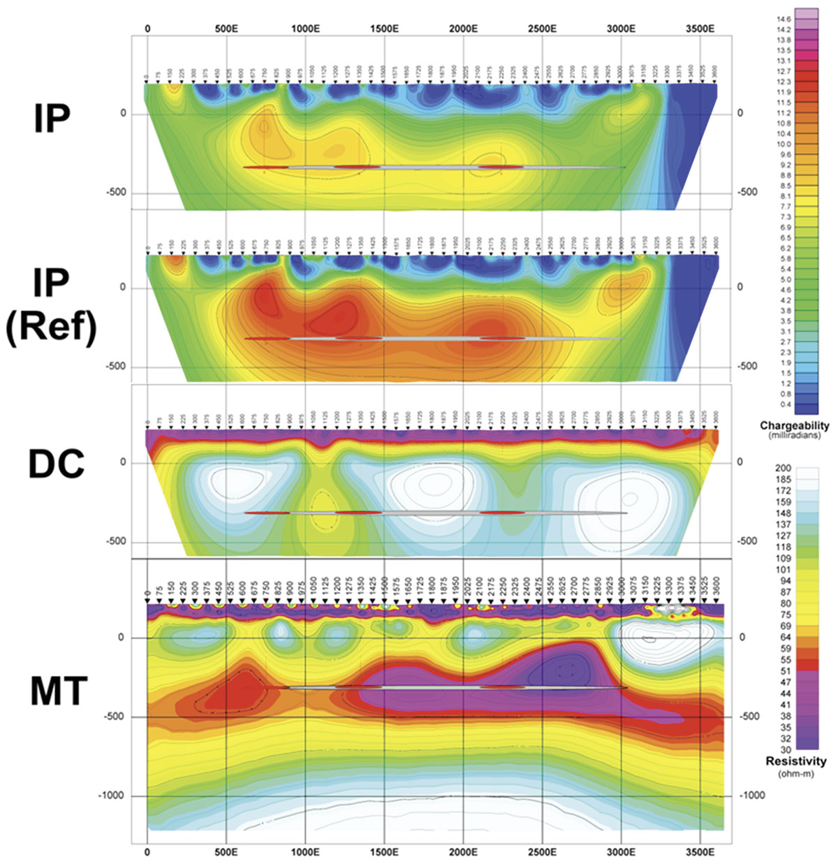
Two IP inversion models are presented, the IP calculated using the inverted DC model (IP Ref, Figure 15, upper middle panel) and the IP calculated assuming a constant resistive half-space (IP, Figure 15, upper panel). The results from the two inversions are remarkably similar suggesting that the anomaly locations are real and consistent in spatial location.

The Induced Polarization (IP) response is most interesting in that there is a consistent chargeability anomaly associated with the lateral extent of the gas pool, but generally at a shallower depth (particularly to the west) between 10 metres and 100 metres and coincident to the east (Figure 15, upper panels). The observed responses may be the result of any one or a combination of the following: increased porosity and hence increased gas accumulation; presence of diagenetic sulphide mineralisation resulting from the reaction of gas/hydrocarbons interacting with the overlying sedimentary units; or shallower, hydrocarbon/gas trap sequences in the geologic section. Interestingly, the surface clay layer shows little or no chargeability response in the IP model.

In this locale, it appears that the gas pool can be defined not only by a decrease in the local resistivity (increased conductivity) in the MT inversion model at depth, but also by an associated IP chargeability response. Controls on the emplacement of the gas pool may also be determined from the data. The relationship between the apparent basement uplift and gas pool requires further study.

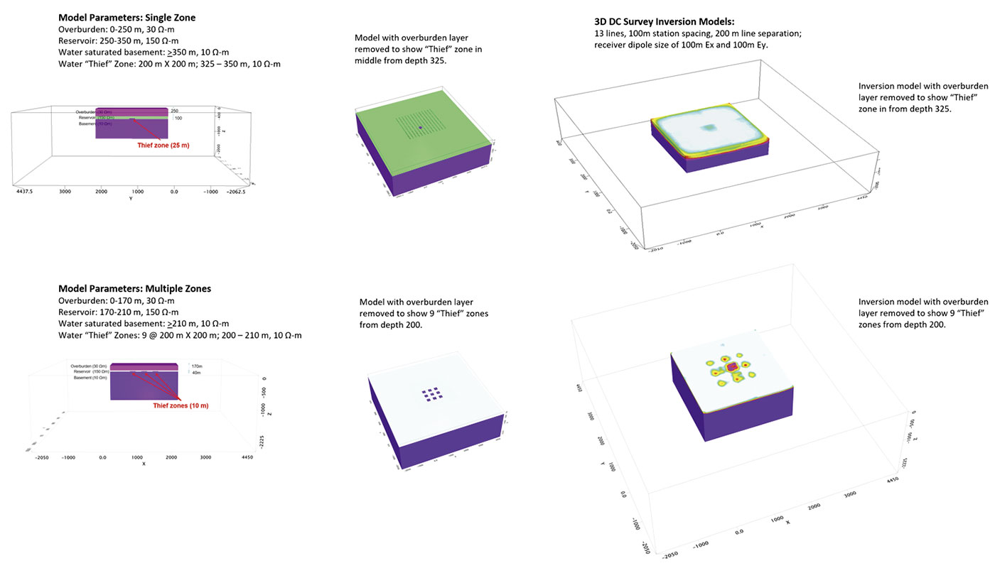
A third example illustrates the potential application of DCIP and MT to map/monitor heavy oil reservoirs to distinguish between water and bitumen rich zones. Forward modeling as illustrated in Figure 16 strongly suggests that the resistivity methods, particularly in 3D, could be effective.

Conclusions

The DC (resistivity) and IP (chargeability) methods have been extensively used for decades in mineral exploration, and to a much lesser extent oil and gas exploration. More recently the MT resistivity method has become a popular tool due to its ability to image to great depth and is routinely used to target wells for industrial scale geothermal power plants.

MT offers opportunities for the combination of methods and integration of resulting datasets. For example, in mineral exploration DCIP can provide high resolution images of shallower ore bodies, with MT adding the deeper underlying tectonic and feeder system details to the geological model. In oil and gas basins MT can provide data to somewhat fill in the seismic image gaps caused by factors such as overlying volcanics or permafrost, or near surface karsting.

Acknowledgements

Much of the material discussed is the result of the hard work and diligence of the interpretation staff at Quantec, namely Dr. Mehran Gharibi and Dr. Benoit Tournerie, and the excellent work by the numerous field crews and processors who have acquired and processed the data. Permission to show data from the Santa Cecilia Project of the Cerro Grande Mining Corporation and from the Michigan Basin project of Torque Energy Limited by David Nelms and Ian Colquhoun is greatly appreciated.