Application of Full Zoeppritz AVO Inversion for Delineating Porous Sand Geobodies Over Aquistore Seismic Survey

We used 3D seismic data from the Aquistore deep saline CO₂ storage project survey, southwest of Estevan, Saskatchewan, Canada, using seismic amplitude variation with offset (AVO) inversion and lithology prediction workflows to delineate the porous sand units across the survey.

Throughout this work, we used both Aki-Richards three-term approximation to Zoeppritz and the full Zoeppritz equations to derive the AVO inversion outputs and demonstrated that the results using the full Zoeppritz method were superior. We then used the better seismic inversion results, derived by means of the full Zoeppritz method, to identify and separate the sand units from other lithologies (carbonate, shale, sandy shale, or mixed). Ultimately, we designed a porosity estimation function and visualized good porous sands geobodies across the seismic survey.

Introduction

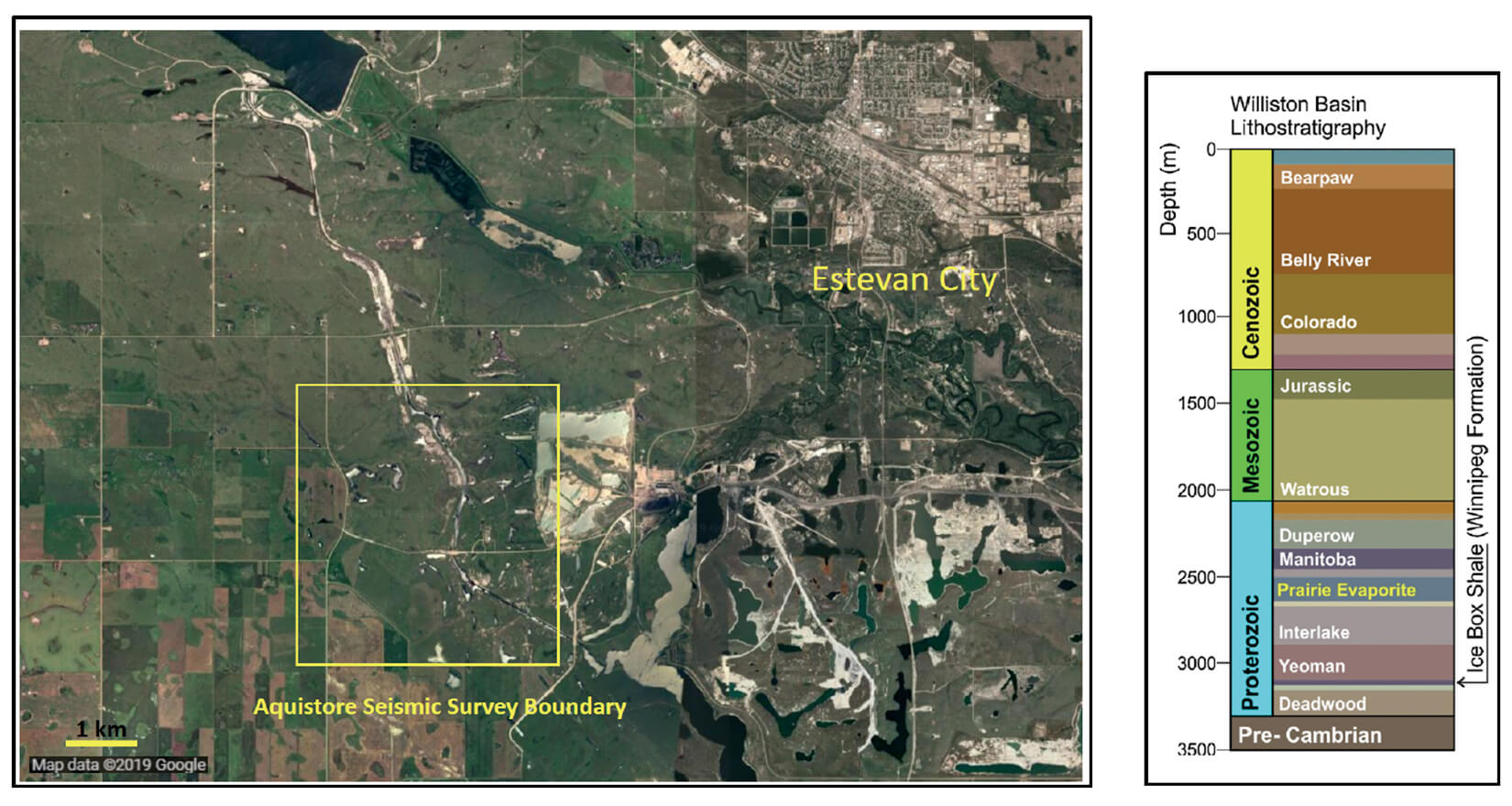
Aquistore, a deep saline CO₂ storage research and demonstration project, is located southwest of Estevan, Saskatchewan, Canada. The Aquistore CO₂ storage site is aimed at demonstrating that CO₂ storage in deep saline geological formations is a safe solution for emissions reduction. The Winnipeg and Deadwood formations, which constitute the deepest units within the sedimentary sequence of Williston Basin, have been chosen by the Aquistore project as the target zone for CO₂ injection. The Deadwood Formation is a regionally extensive sandstone of variable grain-size that contains intervals of silty-toshaley interbeds. The overlying Winnipeg Formation comprises a lower sandstone called the Black Island Member and an upper shale, the Icebox Member, which would form the primary seal to the storage complex. In the area near Estevan, this storage unit is about 3,200 m deep. Figure 1 shows Aquistore seismic survey location and generalized stratigraphy at the Aquistore site.

We used seismic inversion and lithology prediction methods to delineate porous sand units. Prestack time-migrated (PSTM) data (gathers and stacks), a product of 2012 processing, were used as one of the inputs to the inversion. Low-frequency models and seismic extracted wavelets were other inputs for running the inversion workflow.

Seismic Well Ties

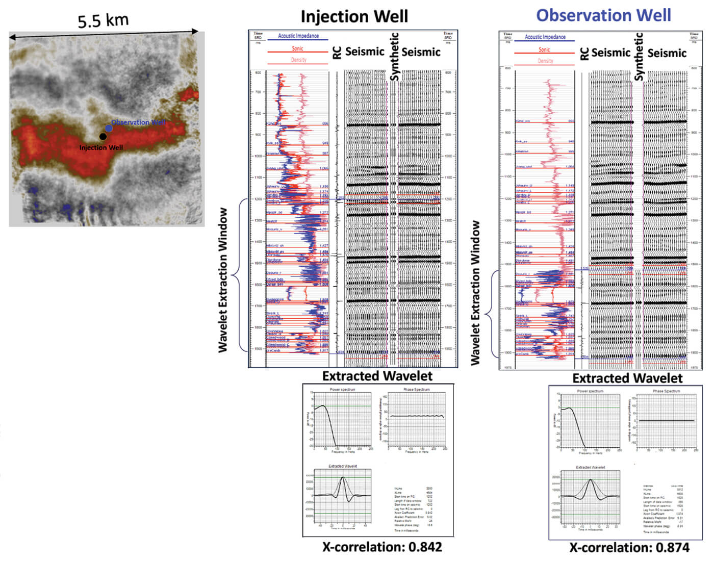
The PSTM stack volume as well as sonic and density logs were used to establish the seismicto- well ties for the injection and the observation wells. Synthetic traces were generated by convolving extracted wavelets with reflectivity derived from well log data.

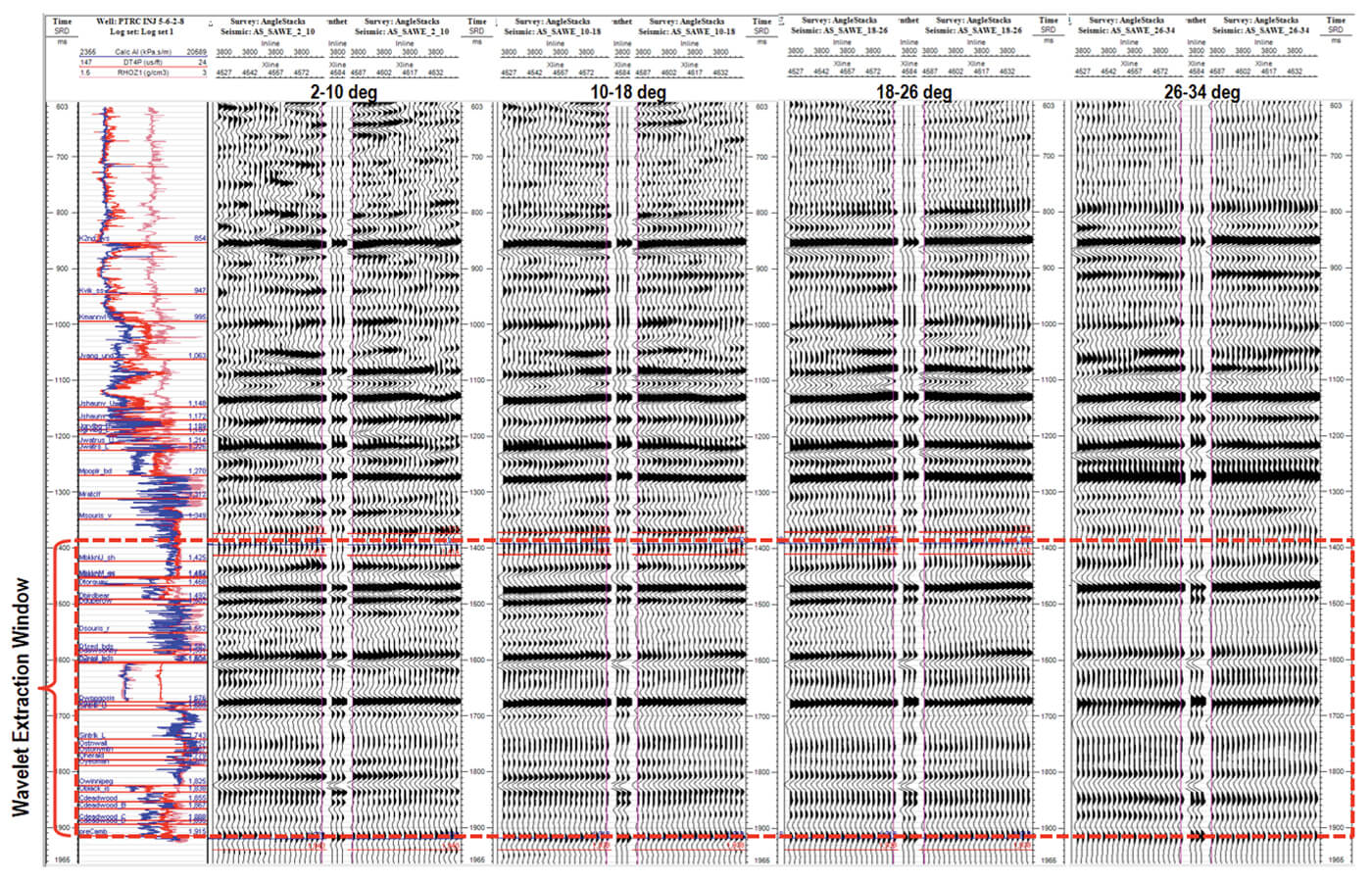
Figure 2 represents the well-to-seismic tie and the extracted wavelet for the injection and observation wells. The synthetic correlates quite well with the seismic data, as demonstrated by the correlation coefficients which are 0.842 and 0.874 for the injection and observation wells. Such high correlation between logs and seismic data suggests that plausible multiples were effectively suppressed during the seismic processing.

Angle Stacks Decomposition

The supplied PSTM gathers were normal moveout (NMO) corrected using the processed seismic interval velocity. Five common image gathers were selected from various locations in the survey for analyses to determine the optimal angle stacks ranges. The generation of the angle bands is performed using reconfiguration of Snell's law to relate the angle of incidence into time, offset and velocity, as described by Walden (1991). The seismic velocity used for angle stacks decomposition was obtained through number of semblance velocity analysis followed by anisotropic velocity fine tuning.

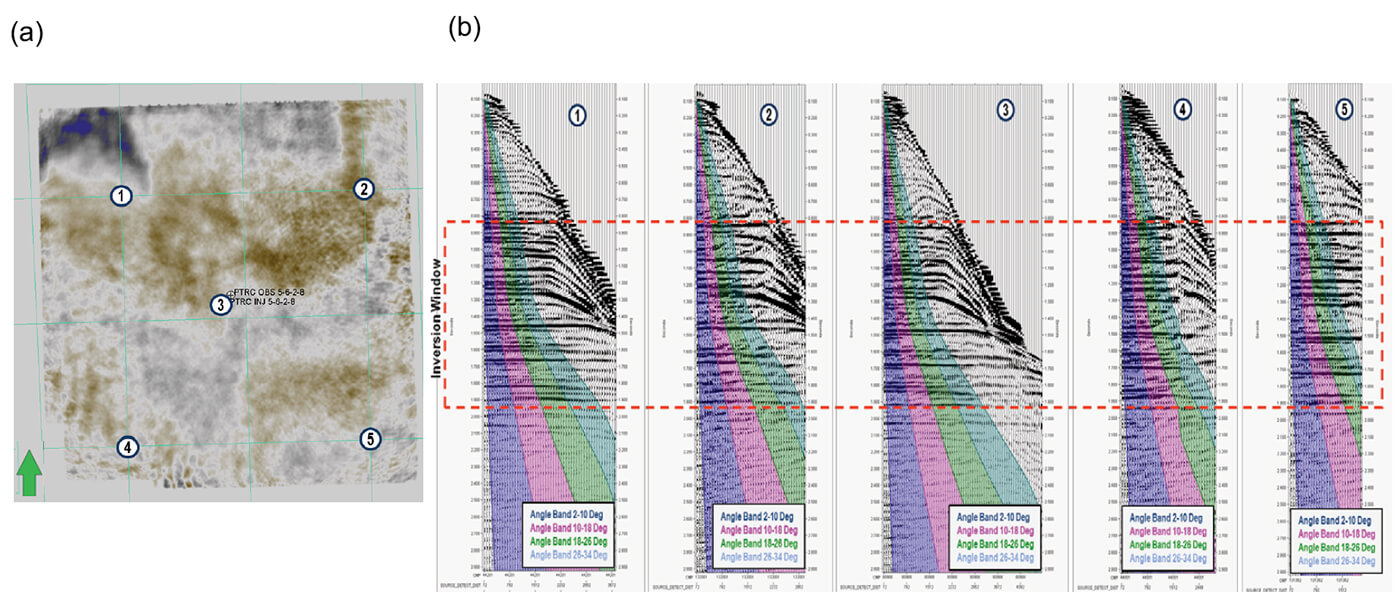
Figure 3-a displays the selected gathers locations. Based on the testing, four angle bands, each with a bandwidth of 8°, were selected for use in the amplitude variation with offset (AVO) inversion. Figure 3-b shows the inversion window, an approximately one second time window that covers the target reservoir, indicated by the red dashed-line rectangle, and gathers with angle bands of 2-10°, 10-18°, 18-26°, and 26-34° are overlaid.

The prestack seismic data were decomposed into the above-mentioned angle stacks. Conditioning of the angle stacks was performed prior to executing AVO inversion.

Angle Stacks Conditioning for AVO Inversion

Seismic data conditioning before inversion is vital to properly invert for rock properties. In this project, we applied space-adaptive wavelet equalization (SAWE) for better stability and consistency of the angle stacks wavelets and non-rigid matching (NRM) to better align reflected boundaries across the angle stacks.

Space-Adaptive Wavelet Equalization (SAWE): Stabilizing the seismic wavelet was performed by estimating and compensating for space-variant and space-invariant components. The wavelet was assumed to be composed of the following components:

• Source: Spatially stable arbitrary phase
• Propagation: Space-variant minimum phase
• Receiver: Spatially stable arbitrary phase
• Processing: Spatially-invariant arbitrary phase

The method consists of taking the non-minimum phase component of the wavelet, extracted at the well location and adapting its phase and amplitude spectra to include the minimum-phase spatially varying propagation component. The wavelet processing operators were individually designed to cancel the locally estimated phase components.

An additional operator task was to normalize the wavelet spectral amplitude to a common spectrum, derived from the signal and noise analysis of the input data within the desired inversion window. The resulting seismic data after SAWE should demonstrate a wavelet closer to zero phase, with similar amplitude spectra among traces.

Wavelets before and after SAWE were extracted from the angle stacks at the injection well. As shown in Figure 4, the extracted wavelets after SAWE are more consistent and closer to the desired zero-phased wavelet.

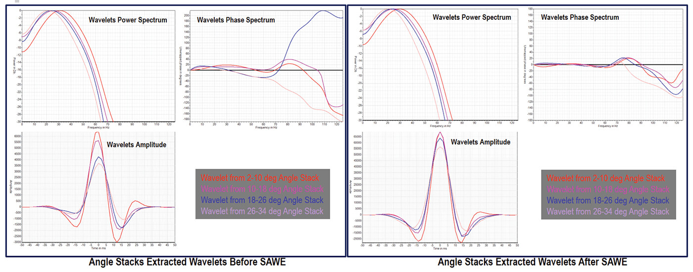
Figure 5 shows good well ties for the angle stacks, providing further confidence for subsequent seismic inversion.

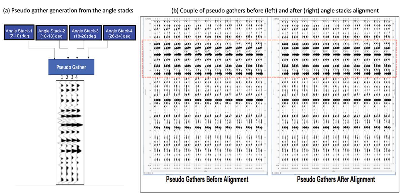
Angle Stacks Alignment: The non-rigid matching (NRM) technique was used for the time alignment of the angle stacks. The technique calculated the vertical displacement of each sample between the 10-18° reference angle stack and the input volume over a given time window, while minimizing any residual NMO. The vertical displacements were then filtered and applied to the input angle stack volumes to align them to the reference angle stack volume. The process was performed over a time window covering the inversion target. Angle stacks 2-10°, 18-26°, and 26-34° were aligned to the 10-18° reference angle stack.

To quality control (QC) the alignment step, pseudo-gathers were derived from the four angle stacks before and after the alignment. Figure 6-a shows the pseudo-gather generation workflow and Figure 6-b shows a few gathers before and after the alignment process. As demonstrated, the pseudo-gathers after the alignment show a better flatness of the events.

The conditioned angle stacks (after SAWE and alignment) were used as an input to the AVO inversion workflow.

Low-frequency Model Building

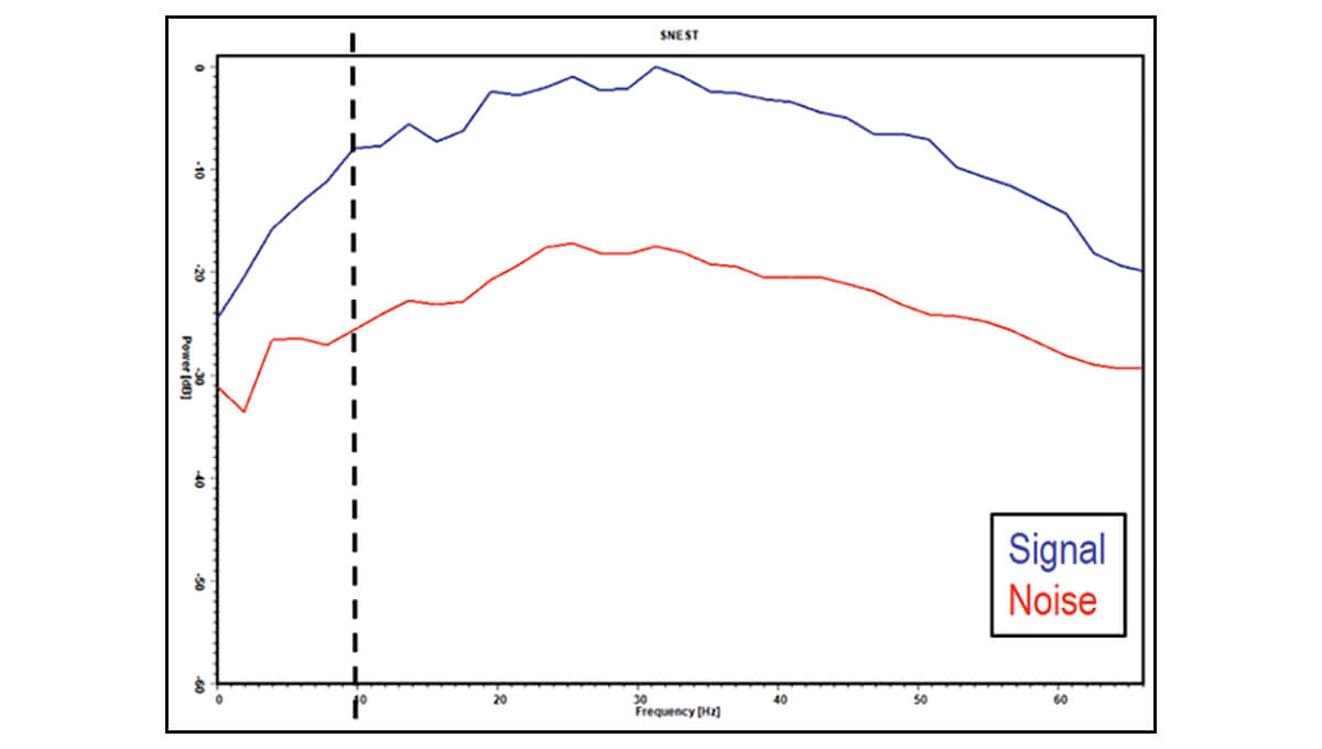
The low-frequency model (LFM), or the prior model, is the starting point for the inversion iteration process. It was generated by laterally extrapolating the low-frequency trend of the wells, constrained by the seismic horizons and other guide information if needed. The LFM role was to fill the lowest frequencies that are generally very weak or absent in seismic data. Filtered logs with a 10-Hz high-frequency cut were used for LFM construction. This filter choice was made based upon the frequency content analysis in the seismic data within the inversion window. Figure 7 shows signal- and noise-estimated frequency plots within the inversion window. As shown, signal is weak below 10 Hz within the seismic data and, hence, LFMs were constructed using log data to contain up to 10 Hz. It should be noted that seismic data may even contain weak signals below 10 Hz. The inversion process uses resolvable low-frequency events in seismic data before reverting to LFM.

AVO Inversion Workflow and Method

The inputs into the simultaneous AVO inversion kernel were the aligned angle stacks, each with its associated extracted wavelet, and low-frequency models for acoustic impedance (AI), Vp/Vs, and density.

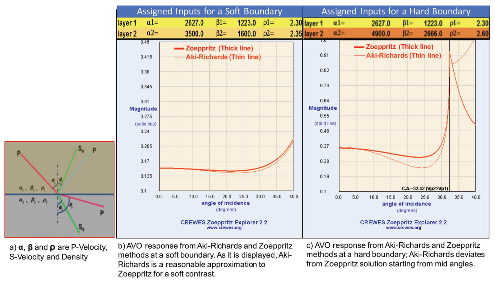
Herein, in addition to the three-term Aki-Richards approximation that is routinely used to derive AVO inversion results, a newly developed full Zoeppritz method was also executed. The new method is designed to capture a better dynamic from seismic data, as the common method (Aki-Richards approximation) normally works well for layers with soft contrast; however, it may not provide good estimates for layers with hard contrast and long-offset gathers.

For a soft boundary, there are relatively small differences between elastic attributes for the top and the layers below associated with the boundary. On the contrary, a hard boundary demonstrates larger differences for elastic attributes, such as P- and S-velocities and density. Figures 8-a and 8-b, illustrate synthetic AVO responses, made using both Aki-Richards and Zoeppritz equations, for typical soft and hard boundaries. As shown in the figures 8-a and 8-b, the Aki-Richards response follows the full Zoeppritz AVO response exact solution for the soft boundary. The approximations, however, deviate from the full Zoeppritz solution for the hard boundary, and this suggests that the three-term Aki-Richards response may not be the optimum equation to analyze real AVO signatures and, consequently, to solve elastic attributes from seismic data.

AVO Inversion Results

An important inversion QC is the comparison between inversion results and the measured logs at the well locations. Figures 9 and 10 show the comparison between inversion-derived (AI, VpVs ratio, and density) and the injection well log measured properties. Figure 9 represents the inversion result using the Aki-Richards response and Figure 10 displays the results from the full Zoeppritz methods. For each property, the left panels show the well log curve that is inserted into the inversion volume and the right panel compares inversion output (blue curve), well log (red curve), and LFM (green curve). In these displays, a 70-Hz high-cut filter is applied on the well logs so that the frequency content of the logs and inversion are comparable.

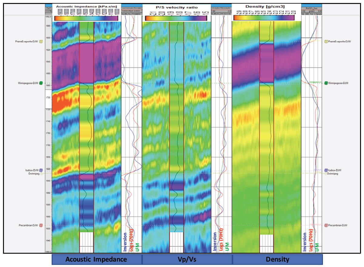
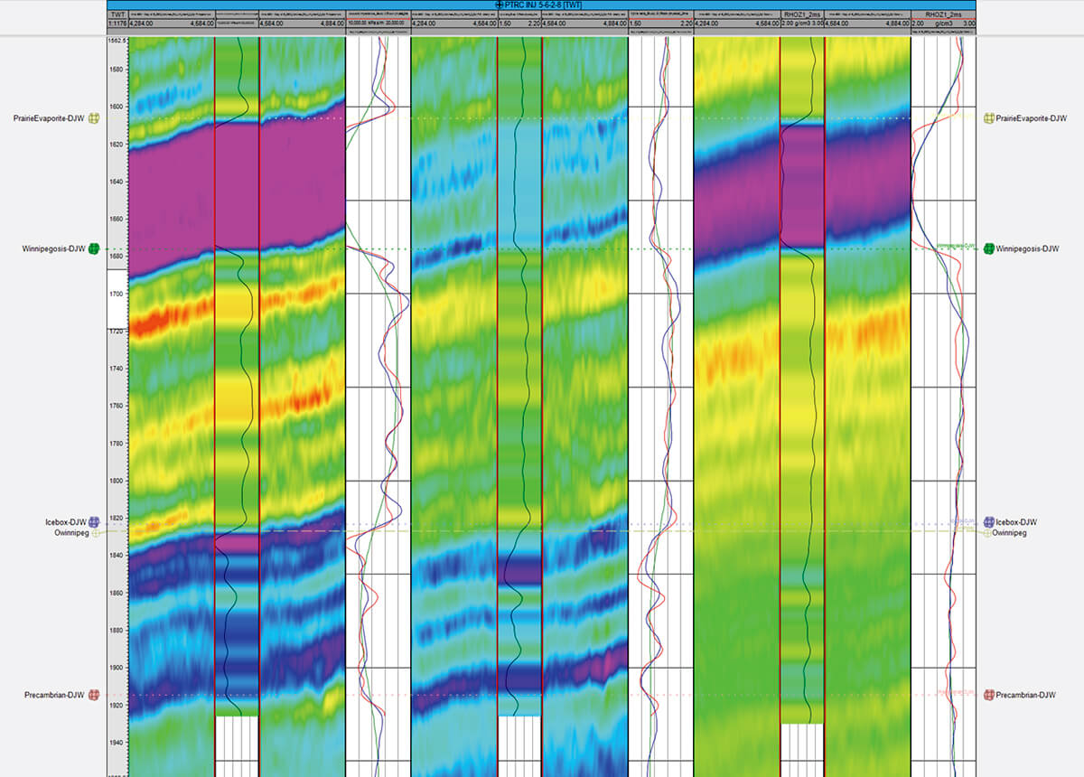
Both methods produced good estimates of AI and VpVs ratio; however, the full Zoeppritz results better captured the true dynamic of the properties from seismic data. The density estimations from both methods do not contain much variation and mostly follow the LFM.

That was probably because only up to 34° of far incident angle was incorporated in the AVO inversion, which is not sufficient to capture density variation from seismic data, especially if the density of the target interval only manifests subtle changes.

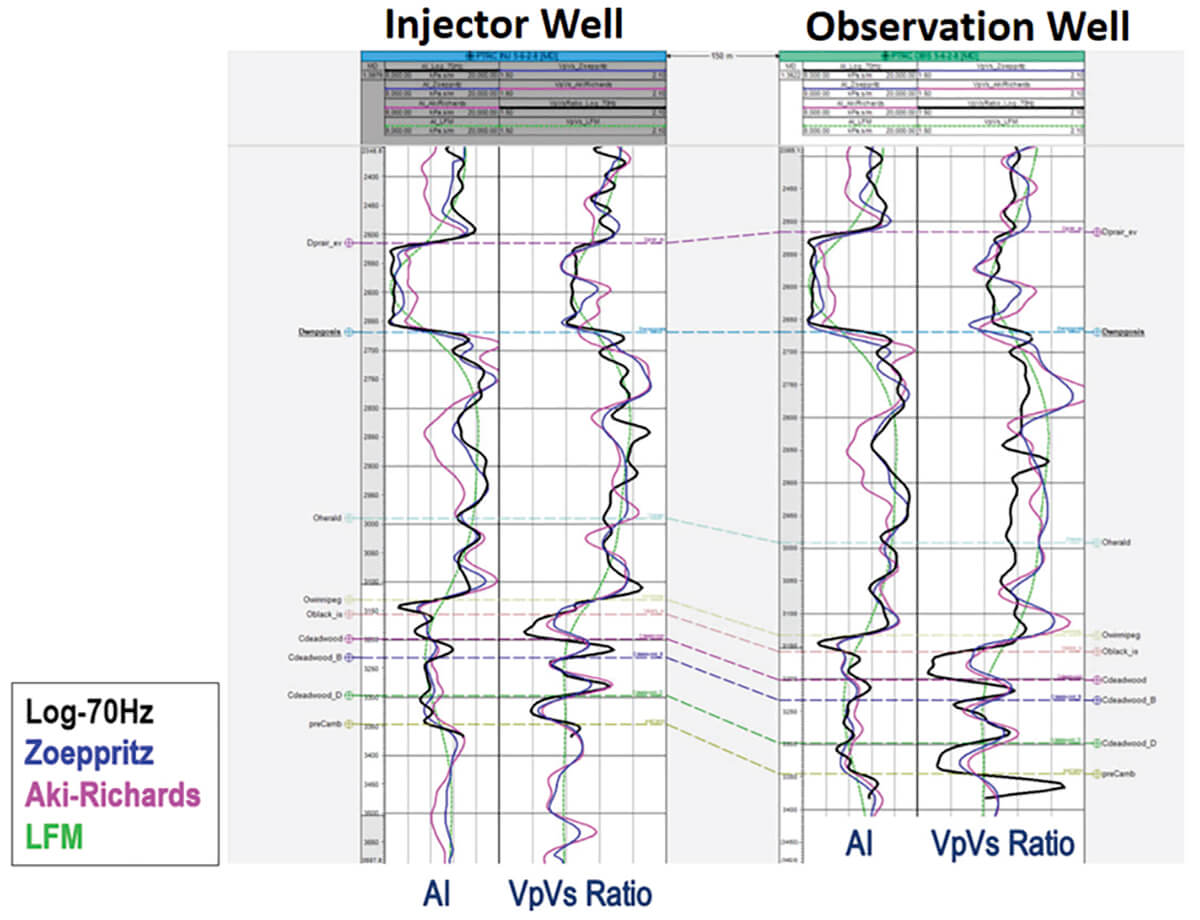
Figure 11 compares the AI and VpVs ratio inversion results from both methods (Aki-Richards and full Zoeppritz) for the injection and observation wells. The 70-Hz filtered logs are displayed in black, Aki-Richards estimation in pink, and full Zoeppritz in dark blue colors. As shown, the estimated properties from the full Zoeppritz response correlate better with the actual logs measured values. Such improvement is more obvious in AI and less obvious in the VpVs ratio; however, for both properties, the full Zoeppritz method provided a better estimation from seismic data.

We then used the inversion derived properties from the full Zoeppritz approach for lithology prediction.

Lithology Prediction

Cross-plot analysis was performed using AI, Poisson’s ratio (PR), and petrophysical volumetric logs from the injection well over the Winnipeg-Precambrian interval. The aim of cross plots was to identify the likelihood of separability of litho-classes, defined on key petrophysical rock properties, using the elastic rock properties. If such separations are observed, we could then employ inversion-derived elastics attributes to predict Continued on Page 6 Injection Well Observation Well lithologies across the seismic survey.

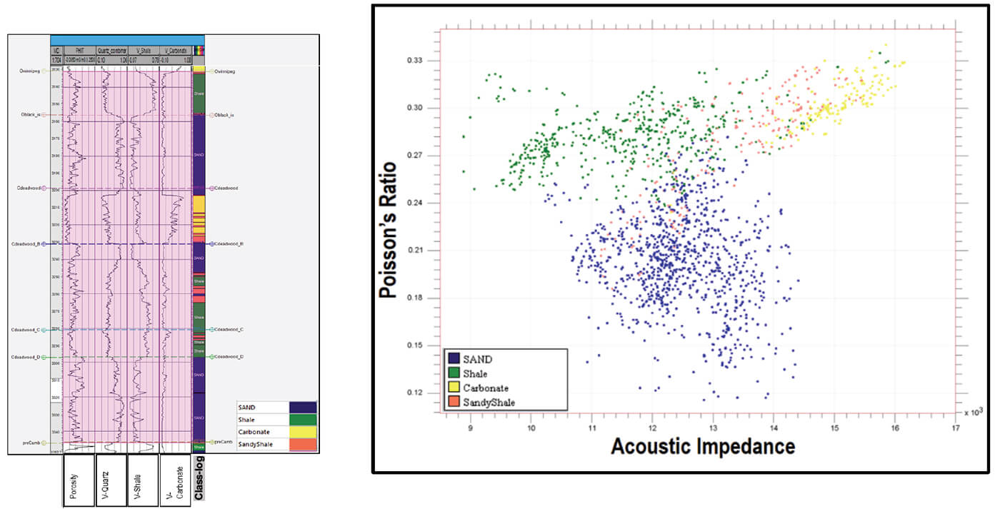
Figure 12 illustrates AI-PR cross plots that are color-coded with volume of quartz, volume of shale, and volume of carbonate, 12-a, 12-b, and 12-c, respectively. It is noticeable that units with dominant quartz content exhibit low PR values. Conversely, shale-rich units exhibit high PR and relatively low AI values. Also, carbonate units exhibit the highest AI (compared to the other lithologies), and relatively high PR values.

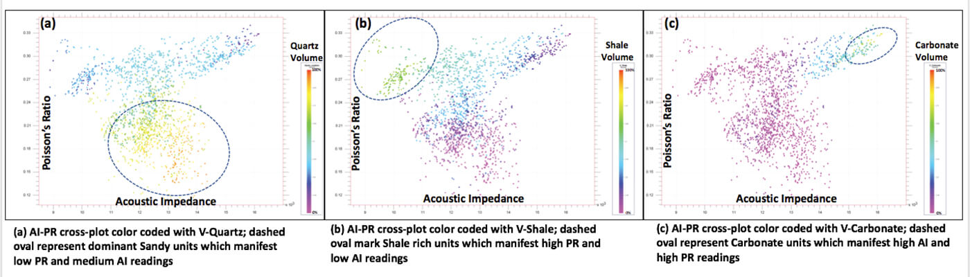
We then classified the following four litho-classes:

1. Sand class: V-quartz > 50%
2. Shale class: V-shale >45%
3. Carbonate class: V-carbonate >35%
4. Mixed class (mostly sandy shale): The rest of the points that did not meet criteria for any of the above classes

The discrete log that contains classification at each depth was referred to herein as the class log. Figure 13, left side, shows volumetric logs and the class log, right side, also demonstrates the AI-PR cross plot color-coded with the class log in the Winnipeg-Precambrian zone.

Next, a two-dimensional probability density function (PDF), using AI and PR logs, was established from a cluster analysis on the AI-PR cross plot. Finally, the established PDF was used to transform seismic attributes, using the Bayesian estimation theory, into the lithology classification volume as well as probability volumes associated with each litho-class. The following were the cubes generated with lithology prediction:

• Class cube (with discrete values; Class-1: sand, Class-2: shale, Class-3: carbonate, and Class-4: sandy shale)
• Probability cube for sand class
• Probability cube for shale class
• Probability cube for carbonate class
• Probability cube for sandy shale class

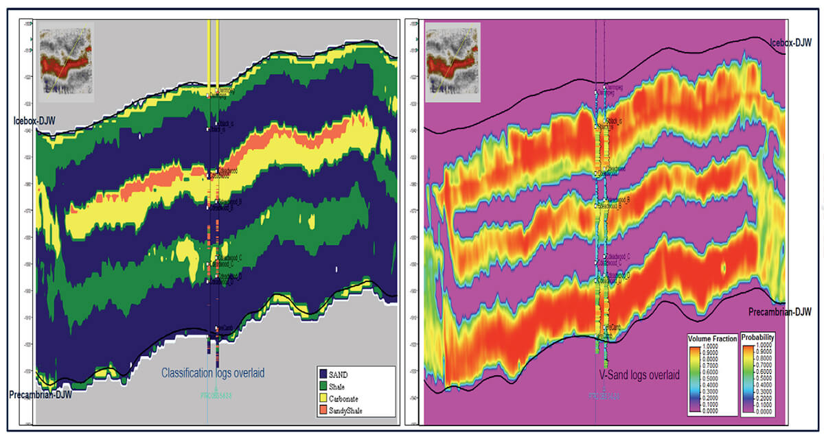
Figure 14 shows arbitrary lines connecting the injection and observation wells from the class cube, left, and probability for sand cube, right. The logs (class logs and V-sand logs) are overlain to cross-check the cubes from lithology prediction with the logs. Even though the logs and the seismically predicted cubes have very different inherent resolution, the derived lithology prediction results correlate fairly well with the class logs for most of the intervals. Also, as demonstrated on the right side of Figure 14, there is a good correlation between the V-sand log and the predicted probability for the sand cube. This was aligned with the primary study focus, porosity estimation within sand units, and we further used the sand probability and acoustic impedance volumes to identify and estimate porosity for sand units.

Porosity Estimation

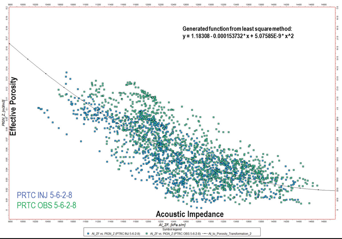
The AI attribute is routinely used to generate porosity estimates from seismic data. Logs from two wells (injection and observation) were used to derive the relationship between AI and porosity attributes. The ultimate focus was to have porosity estimation within the sand units and, hence, the relationship between AI and porosity logs for only the classified sand points were examined. Figure 15 shows the AI-porosity cross plot for the sand units from the two wells and the derived AI-to-porosity function is overlaid in black.

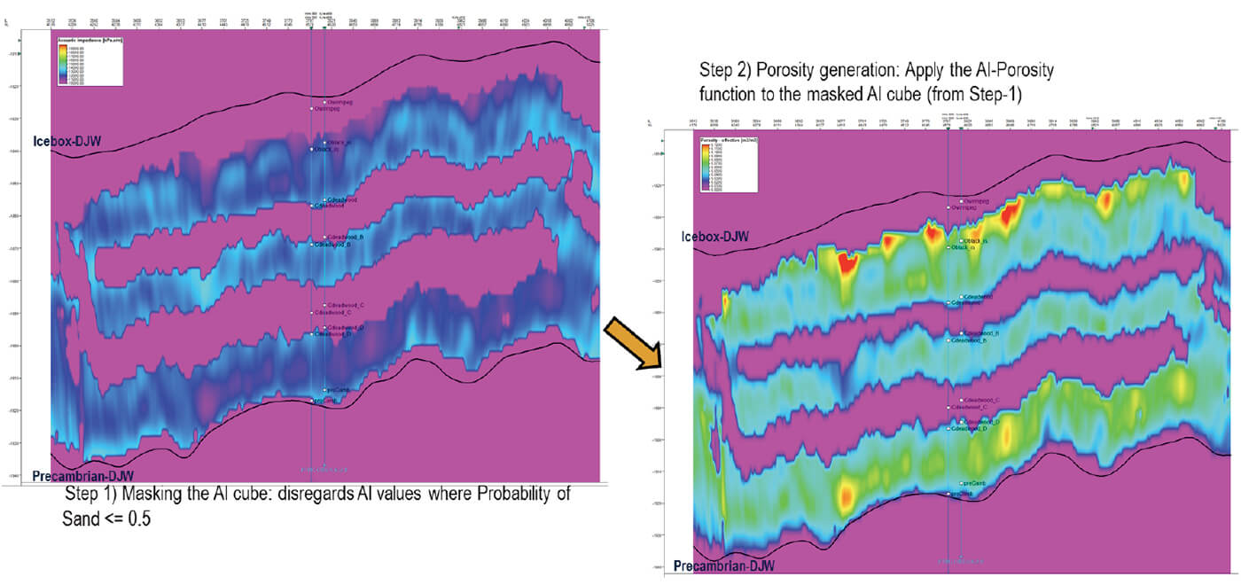
The derived function was used to transform the AI cube from the seismic inversion workflow into porosity cube in two steps: Firstly, the combined sand probability cube was used to mask the AI cube where the probability percentages were less than or equal to 50%. By doing so, all the lithologies other than sand units were discarded within the AI cube. Secondly, the AI-to-porosity transformation function was applied to the masked AI cube. Figure 16 demonstrate the two-step process for porosity estimation within the sand units.

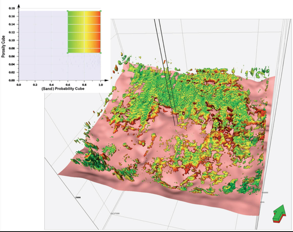
Sand Geobody Extraction

The seismically derived porosity and the sand probability cubes were used jointly for sand geobody extraction in the Deadwood-C to Precambrian zone. The two cubes were rendered for porosity values greater than 7%, and the sand probability greater than 60% (Figure 17). It can be observed that, for the Deadwood-C to Precambrian zone, the porous clean sand units are mostly located in the northern part of survey.

Conclusion

In this paper we utilized both Aki-Richards three-term approximation to Zoeppritz and the full Zoeppritz equations to derive the seismic inversion outputs. We compared the outputs and used the better ones, obtained from full Zoeppritz equation, for discriminating porous sand units across seismic survey. Having the porous sand visualized, by means of seismic, will help further planning for drilling wells and/or optimizing injections.

Acknowledgements

The project was initiated by the Petroleum Technology Research Centre (PTRC) in Regina, and involved a consortium of industry, government, and research organizations. The author thanks PTRC and Schlumberger Canada for permission to publish this work, with special thanks to Don White, Eric Nickel, George El-Kaseeh, and Mark Piercey for their support and contributions to this work.