An Overview of Microseismic Acquisition Project Management

In the past decade, the boom of stimulation and production from the unconventional reservoirs have made microseismic monitoring a commonly used technology in the petroleum industry. However, the recent business challenges faced by the petroleum industry have amplified the need for cost optimization while achieving the maximum benefits from a microseismic project. Understanding the project life cycle structure is fundamental to achieving the desired cost to benefit ratio. Like any project, a microseismic acquisition project also follows the generic life cycle structure (PMBOK Guide, 2013)

• Starting the project
• Organizing and preparing
• Carrying out the project work
• Closing the project

Initiation processes involve defining the project scope and high-level objectives, estimating the available financial resources, identifying internal and external stakeholders, and obtaining the necessary authorization to start the project. Stakeholder involvement during the project initiation helps in creating a shared understanding of the success criteria which improves the acceptance rate of the expected deliverables. Planning processes are performed to define and refine the objectives, and outline the course of action required to successfully achieve those objectives. Execution processes are performed to complete the planned work and take up a large portion of the project budget. Throughout the project, monitoring and controlling processes are required to evaluate the performance of the project and to identify deviations from the planned work that require further attention. Finally, the closing processes are performed to formally complete the project (PMBOK Guide, 2013). In this paper, we outline microseismic data acquisition in terms of project life cycle and process groups to demonstrate how understanding the different processes involved can help in achieving maximum benefits while optimizing the cost.

Initiation

Microseismic monitoring may be required for any of the following reasons (Cipolla et al., 2012):

• Real-time monitoring control of hydraulic fracturing
• Understanding the induced and existing fractures dimensions, orientations and network complexity
• Monitoring and controlling out of zone fracture growth
• Identifying unfractured caprock (absence of microseismic events)
• Use of microseismic data in integrated interpretation with other geological, geophysical, petrophysical and other engineering data
• Use of microseismic data in reservoir engineering workflows and geomechanical modeling
• Use of microseismic data in future well planning
• A research project to test a new instrument or survey configuration

After the need of a microseismic survey is established, it is important to estimate the costs involved and the available resources. Identification of key stakeholders involved in the project is also important at this stage. The key stakeholders (geologist, geophysicist, reservoir and production engineers, accounts/financial and technical managers, etc.) can be from within the same organization and/or from a partner organization. Other important stakeholders are the contractors who will be involved in completing several tasks during the course of the project. A high level knowledge of available contractors, type of instruments, the expected deployment of the receivers (e.g. on the surface, in shallow boreholes, in boreholes near the reservoir depth, or a hybrid combination of surface and borehole configuration), duration of the survey, the required permits and key deliverables are also useful at this stage. Stakeholder involvement during the project initiation helps in defining a project scope which creates a shared understanding of the success criteria. A project is officially initiated once a designated authority (senior management) approves the project scope and budget. It is also important to assign a central point of contact (a technical person in charge or a dedicated project manager) to keep track of the project progress and performance.

Planning

Planning is the most important stage in the acquisition of a microseismic survey. In this stage, the high level scope and objectives defined in the initiation stage are carefully reviewed, assessed, and decomposed into more easily achievable objectives. A suitable course of action is then planned to achieve the objectives in a timely and cost effective manner. Gathering necessary information from previous case studies, lessons learned and best practices is important. Key information may include any incident on the field (e.g. equipment failure, noisy sources, or a health, safety and environment (HSE) event), type of geology and the associated microseismic activity, type of well completion, injection rates, and the source-receiver configuration (Freudenreich et al., 2012). The decision of whether to place receivers in downhole or surface settings depends on several factors such as the objective of the survey, economic constraints etc. It is important to realize that both surface and downhole monitoring have their pros and cons. Downhole microseismic monitoring has a basic requirement of monitoring well(s) near to the treatment well. Often the monitoring well is a production well but it can also be the treatment well (Maxwell, 2014). Depending upon the case, factors such as the production loss, effect of elevated background noise during injection on data quality or the cost of drilling new monitoring wells (if none exists) require careful consideration. Although the placement of receivers at the reservoir level helps in recording high signal to noise ratio (S/N) data, the location accuracy of microseismic events generally decreases away from the observation well. Single linear receiver array deployed in a vertical well has a small angular aperture and provides poor focal coverage. Multi-well deployments are therefore required to retrieve important information about source mechanisms, to achieve accurate event locations, to obtain a high resolution image of the fracture(s) or to improve the quality of recorded data. On the other hand, surface and shallow buried arrays provide good coverage of the focal sphere. Such configurations can also be used in the permanent monitoring. Due to the presence of several noise sources at the surface, S/N of the recorded data is often low. However, deployment of receivers in shallow boreholes (buried grids) can improve the S/N of the recorded data. Additional processing effort is often required to improve the data quality. Cost factor is another key element in the choice of survey configuration, for instance surface receiver geometry will be more economical for monitoring an entire field as compared to the downhole receiver geometry.

Feasibility modeling can also be performed in order to ensure the optimum receiver location. Freudenreich et al. (2012) summarizes the information required for a feasibility modeling study

• Well locations and well trajectories
• Completion diagrams
• Subsurface geology information (i.e. gamma ray (GR), P- and S-wave velocity, and density logs)
• If available, seismic sections (i.e. waveforms, Q-estimates and velocity profiles)
• If available, information from analogue settings (i.e. type of microseismic activity, b-values, magnitude-distance relation, inferred source mechanisms and moment tensors, etc.)

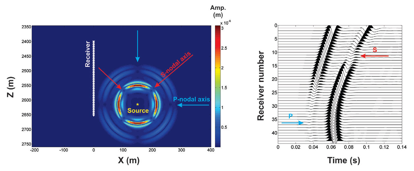
Simple waveform modeling can be performed using the available well locations, well trajectories, velocity models (obtained from sonic logs or from surface seismic) and dominant moment tensor solution from analogue settings to observe the proximity of nodal planes of the expected microseismicity to the receiver array and also to understand the waveform complexity. Figure 1 shows an example of 2-D synthetic waveform modeling of a double-couple source mechanism. In this case, weak P-amplitudes are recorded on the deeper receivers due to the P-nodal axis (plane in 3-D case). Similarly, an S-nodal axis intersects the receiver array at receiver 11, resulting in the S-wave polarity flip above and below this receiver level.

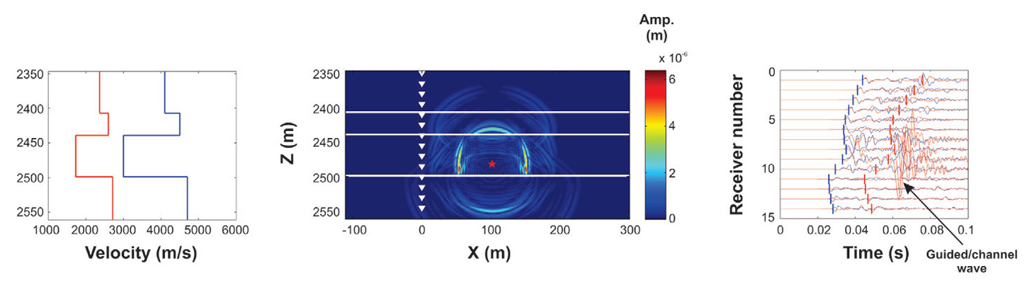
In the field examples, microseismic waveforms may be more complex due to the presence of other noise sources. For example, a guided wave is trapped within the low velocity layer due to the surrounding high velocity layers and is propagated to the receivers placed at the same depth (Figure 2). These guided waves have higher amplitude and their presence may complicate the arrival picking. However, these wave types can be useful in calibrating the low velocity layer. In case it is desired to avoid recording of these channel waves, receivers can be moved to locate above the low velocity layer. Another aspect is the interference of head-waves and direct-waves arrivals that can also complicate the arrival picking. This can also be identified from the waveform modeling and the survey design can be adjusted to avoid the interfering head-waves and direct-waves (Zimmer, 2011).

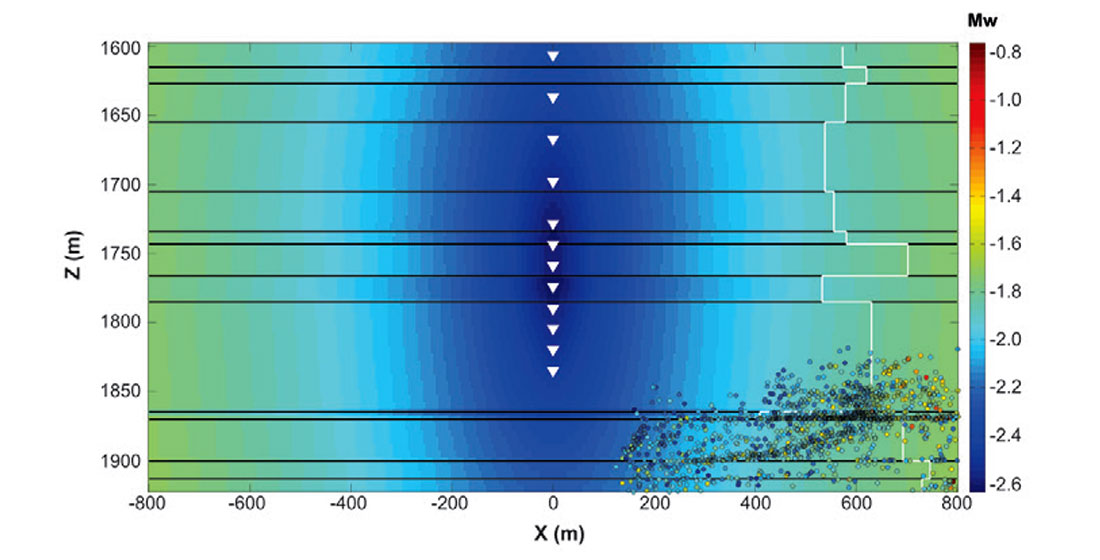
Another concern is related to event detectability with the planned source-receiver geometry. Using the information from analogue settings, a magnitude-distance relation can be used to detect the maximum detectability distance (Zimmer, 2011; Freudenreich et al., 2012; Maxwell, 2014). The b-value statistics can provide information about the type of microseismic activity. In addition, an event detection modeling can be performed for the expected source-receiver geometry. A detectability criterion that relates a threshold value of ground motion velocity to a moment magnitude value can be established using traveltime, Q-value, and some assumptions about background noise level and source directivity (Freudenreich et al., 2012). Figure 3 shows an example of event detectability modeling and the actual results of a microseismic survey overlaid together. In general, the field results agree with the modeling results, which are based on various assumptions about source directivity, Q-value, source-directivity, etc.

In addition to waveform complexity and event detectability, it is important to understand the location accuracy for the planned source-receiver geometry. Grechka (2010) describes a modeling technique based on singular value decomposition (SVD) of Fréchet derivative matrix of modeled traveltimes. The singular values of Fréchet derivative matrix can help in determining whether a microseismic event can be uniquely located from the traveltime data. Figure 4 shows the smaller singular value (S₄) of the Fréchet matrix for traveltime from 16 receivers deployed each in two vertical boreholes. The traveltimes are computed for a layered velocity model. The red color (higher S₄ value) indicates the areas where accurate location of microseismic events will be observed for the geometry in consideration.

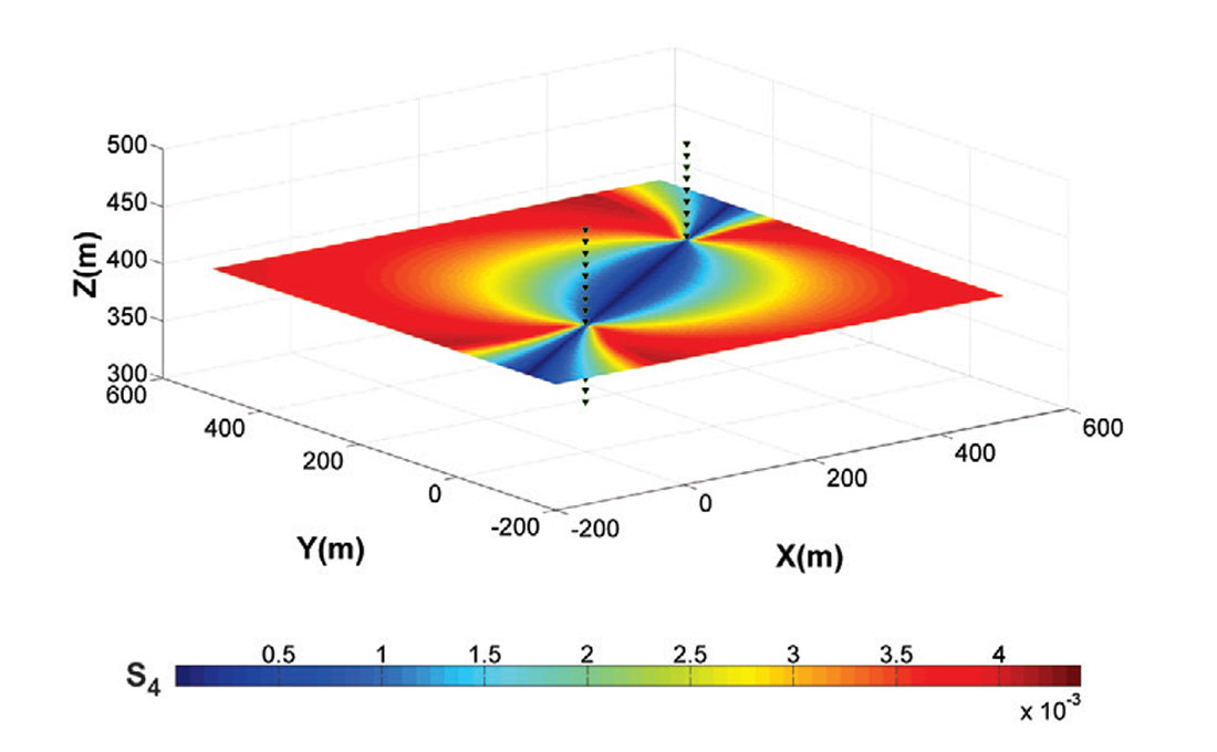
The value of S₄ > 0 indicates that all four quantities (three spatial coordinates and origin time) needed to locate an event are uniquely resolved from the traveltimes only. In the case of S₄=0, additional information (e.g. polarization estimates) is required to locate the microseismic event.

Care is also required in the selection of the correct instrumentation that is suitable for the temperature and pressure conditions at the planned borehole depths and can record the expected signal frequencies (10-1000Hz) with minimal distortion. As pointed out in Maxwell (2014), recorded noise levels are further elevated above background seismic conditions by the noise introduced by the recording system itself and therefore, a properly engineered system with low system noise is desired. Similarly choice between geophones or accelerometers is made based on bandwidth and inherent noise characteristics.

Once the survey planning is finalized (design and the choice of instrumentation/ equipment), a suitable contractor who fits a predetermined criteria (typically in line with optimizing cost to benefit ratio) can be selected through a bidding process to perform the field execution of the acquisition project. Existing quality, health, safety and environment (QHSE) policies can be adopted and implemented during the field execution.

Execution, monitoring and controlling

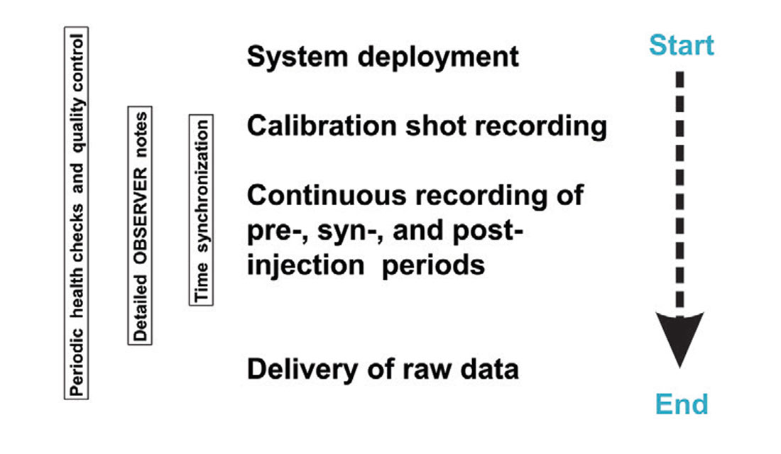
Field execution of microseismic data survey is the process where majority of the budget is expended. Figure 5 illustrates in brief the field execution steps for a microseismic survey, particularly for hydraulic fracture monitoring. First, the recording equipment is deployed in the field as planned and all the assessments are conducted to ensure the functional quality of the equipment. Other QHSE and operational guidelines are ensured to be strictly in place for field activities. It is followed by the recording of pre-injection background activity, calibration shots, syn- and post-injection periods. All the recordings must be synchronized in time to ensure consistency for the data interpretation stage. Other important information (e.g. bad receiver/channel, noise sources, any anomalies during the recording period and recording time for calibration shots, etc.) should be duly noted in the observer notes for use in the data processing stage. Periodic health checks of the recording equipment and the recorded data are required to identify any problems in time. This ensures the recording quality and is also a pro-active measure to find timely solutions or change of course from the planned survey (if required). After the recording is complete, all data plus documentation is delivered in the desired format (Maxwell, 2014).

Closing

The final stage involves project closure, which starts after all the field data acquisition is complete. It requires that data is stored in the correct formats, full documentation about the field activities are prepared and the required deliverables are received from the contractors. As part of an initiative from the Chief Geophysicist Forum of the CSEG to develop standards for microseismic monitoring, Maxwell and Reynolds (2012) present guidelines and minimum requirements for standardized microseismic deliverables. Use of such standardized deliverables will help in proper archiving of data, thus allowing efficient data analysis and abridging exchange of data within the industry. More details on the guidelines and minimum requirements can be found in the above mentioned reference.

Finally, it is always useful to document best practices and lessons learned at the end of each project phase. The acquisition phase of a microseismic monitoring project is considered closed when the data is successfully transferred to processing department. In the next phase, the acquired data undergoes signal processing to estimate the end products (event locations which are used in inferring fracture geometry, dimensions and the stimulated reservoir volume, and the source parameters to be used in geomechanical interpretation). The processing results are then used to produce a final project report.

Conclusions

We outline the microseismic data acquisition in terms of project life cycle and processes. We describe how understanding of different project processes can help in identifying the objectives and optimizing the planning and execution of microseismic survey for maximizing project benefit. Key stakeholders should be involved from the project initiation stage to help define a project scope which creates a shared understanding of success criteria and generally improves the acceptance rate of expected deliverables. Care is required in the planning and execution stage to achieve the optimal cost to benefit ratio.

Acknowledgements

We would like to thank Brazil’s Science Without Borders Program for their support. We are also thankful to the reviewers for improving the quality of this work.