An Inversion Primer

Introduction

Seismic inversion is a technique that has been in use by geophysicists for almost forty years. Early inversion techniques transformed the seismic data into P-impedance (the product of density and P-wave velocity), from which we were able to make predictions about lithology and porosity. However, these predictions were somewhat ambiguous since P-impedance is sensitive to lithology, fluid and porosity effects, and it is difficult to separate the influence of each effect. To perform a less ambiguous interpretation of our inversion results, we must perform full elastic inversion, in which we estimate P-impedance, S-impedance (the product of density and S-wave velocity) and density. The reason for this is that the P and S-wave response of the subsurface is sufficiently different to allow us to see the difference between fluid and lithology effects. We have now progressed to the point where inversion for P-impedance, S-impedance and density is feasible. This article presents both a history of seismic inversion and an overview of the techniques themselves, illustrated by a case study from the Gulf of Mexico.

Seismic amplitudes

The seismic reflection method was developed in the first quarter of the twentieth century and was used initially as a tool for identifying structures, such as anticlines, which could act as trapping mechanisms for hydrocarbon reservoirs. This was done by simply identifying the continuity of the reflections seen on the seismic sections. However, by the 1970s, geophysicists had begun to realize that information was contained in the amplitudes of the seismic reflections themselves. This information could be correlated with porosity changes, lithology changes, or even fluid changes within the subsurface of the earth.

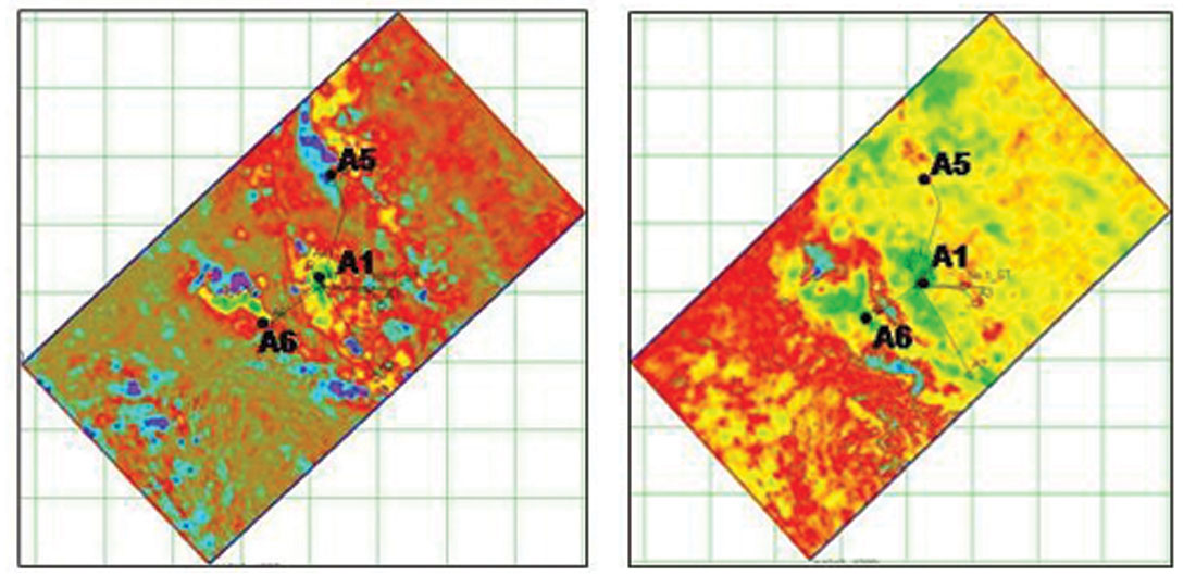
With the advent of 3D seismic recording in the 1980s, we could map the seismic amplitude change over the full extent of a prospect. For example, Figure 1 shows an extracted seismic amplitude map from a recent 3D survey over the Marlin field from the Gulf of Mexico.

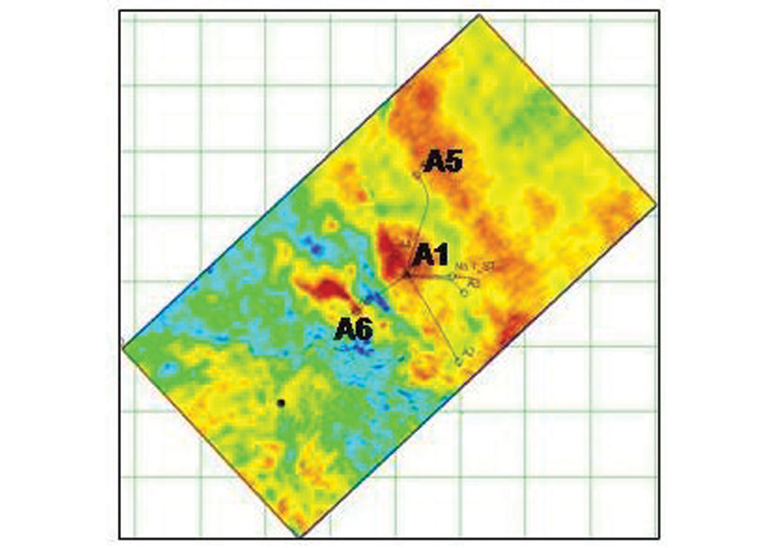
Three wells are indicated on the map in Figure 1: A1, A5, and A6. Well A1 is the initial discovery well, and encountered 150 ft (40 m) of gas at the reservoir level. Well A6 is the updip delineation well, and encountered 80 ft (25 m) of gas sand and over 60 ft (20 m) of water sand at the reservoir level. Well A5 is the downdip delineation well, and encountered no gas sand and 140 ft (33 m) of porous water sand at the reservoir level. Notice that all three of these wells correlate with amplitude anomaly trends (shown by the brown colour on the map), but only two of the wells are producing gas wells. Almost due east of the A1 well are two deviated wells also containing gas but this is not evident from the seismic amplitudes. Seismic amplitude alone is therefore a fairly good indicator that something in the subsurface is anomalous (porosity, hydrocarbon, etc), but is an ambiguous indicator of hydrocarbons.

Seismic reflections and mode conversion

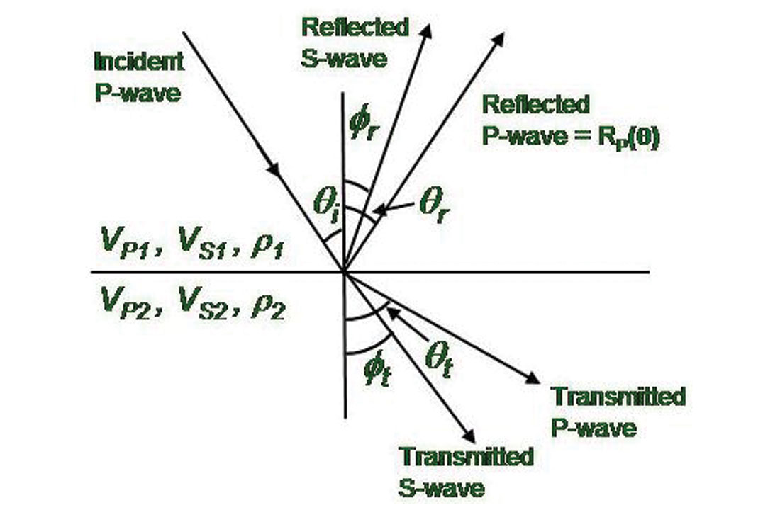
But what does seismic amplitude really mean? The theory of seismic wave propagation, including the reflection and transmission of seismic waves at elastic boundaries within the earth, has been well known for at least a century. These early theoretical studies recognized that both compressional waves (P-waves) and shear waves (S-waves) are generated in an elastic earth (along with many other types of waves, such as Rayleigh waves, Love waves, Stonely waves, etc). Zoeppritz (1919) showed mathematically that if a P-wave was incident on the boundary between two elastic media at an angle greater than zero degrees, reflected and transmitted P and S-waves were created by a process called mode conversion, as shown in Figure 2. Zoeppritz’ equations, which involve the solution of a 4x4 set of linear equations, allow us to compute the amplitudes of each of these waves. Although we will not give the explicit form of the Zoeppritz equations here (see Aki and Richards, 2002, for the complete derivation) a linearized version of the equations will be discussed later in this tutorial.

Despite the early research on different types of elastic waves, the exploration seismic reflection method has traditionally limited itself to the generation, recording and analysis of P-waves alone. (This trend is starting to change, and we are now more commonly recording converted waves or full S-waves using multi-component geophones).

In a typical seismic survey, we generate an incident P-wave using a source such as dynamite, Vibroseis, or a marine airgun. We then record the reflected P-wave as a function of offset, which can be related to the angle θ shown in Figure 2 by the seismic velocity. The result is the seismic shot record. The shot record is then transformed by processing into a common mid-point (CMP) gather, in which the reflection points are grouped around a common midpoint. As we will discuss in a later section of this tutorial, the information contained in a CMP gather contains information about all three physical parameters shown in Figure 2: P-wave velocity (V_P ), S-wave velocity (V_S ), and density (ρ). However, before looking at this process, called AVO, let us consider the more standard seismic process flow, which involves “stacking” the seismic data.

Post-stack seismic inversion

The standard seismic data processing flow involves transforming the CMP gathers into a stacked section, which is an approximation to the zero-offset reflection, in which the angle θ in Figure 2 is equal to zero. (It is an approximation because stacking involves summing over all angles, which means that any angle-dependent processes will get “smeared” together). If we assume that the angle of incidence is zero in Figure 2 and that the layers are flat, the Zoeppritz equations simplify to the more manageable equation given by

where r_Pi is the zero-offset P-wave reflection coefficient at the i^th interface of a stack of N layers, and Z_Pi=_ρiV_Pi is the P-impedance of the i^th layer.

Equation (1) can be used as a simplified model for the reflections (and therefore the amplitudes) found on a stacked seismic section. Lindseth (1988) was one of the first geophysicists to show that if we assume that the recorded seismic signal is as given in equation (1), we can invert this equation to recover the P-impedance as follows:

By applying equation (2) to a seismic trace we can effectively transform, or invert, the seismic reflection data to P-impedance. However, as also recognized by Lindseth, there are a number of problems with this procedure. The most severe problem is that the recorded seismic trace is not the reflectivity given in equation (1) but rather the convolution of the reflectivity with a bandlimited seismic wavelet, plus some additive noise, which can be written

where s_t is the seismic trace, w_t is the seismic wavelet, r_t is the reflectivity integrated from depth to time, * denotes convolution, and n_t is the noise component. The effect of the bandlimited wavelet is to remove the low frequency component of the reflectivity, meaning that it can never be recovered.

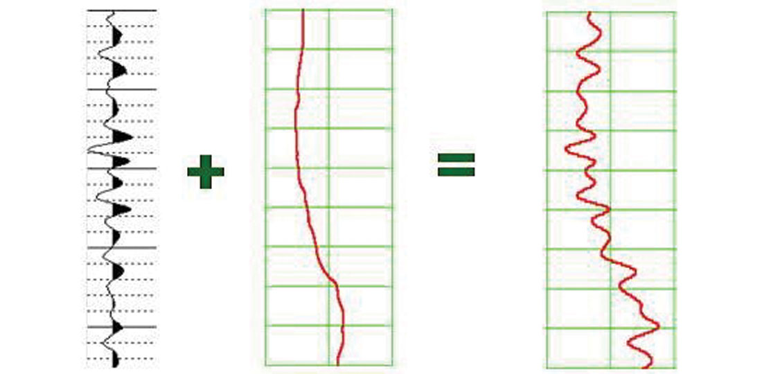
Other key issues in seismic inversion involve removing the noise component and correctly scaling the seismic data. After proper processing and scaling of the seismic data, an intuitive approach to recovering the low frequency component is to simply extract this component from well log data and add it back to the seismic, as shown in Figure 3. In this figure, the trace on the left is the seismic trace after application of equation (2), the trace in the middle is the low frequency component, and the trace on the right is the final result.

A more recent approach to inversion is called model-based inversion, in which we start with a low frequency model of the inverted P-impedance, and then perturb this model until we obtain a good fit between the seismic data and a synthetic trace computed by applying equations (1) and (3). This also assumes that we have extracted a good estimate of the seismic wavelet, which in itself can be a difficult task.

The theory behind model-based post-stack inversion (Russell and Hampson, 1991) is as follows. First, we can show that the small reflectivity approximation for the P-wave reflectivity is given by re-expressing equation (1) as

where i again represents the i^th layer boundary.

If we consider an N sample reflectivity, the noise-free version of equation (3) can be written in matrix form as

where L_Pi = ln(Z_Pi).

Next, if we represent the seismic trace as the convolution of the seismic wavelet with the earth’s reflectivity, we can write the result in matrix form as

where s_i represents the i^th sample of the seismic trace and w_j represents the j^th term of an extracted seismic wavelet. Combining equations (5) and (6) gives us the forward model which relates the seismic trace to the logarithm of P-impedance:

where S is the seismic trace, W is the wavelet matrix given in equation (6) and D is the derivative matrix given in equation (5).

If equation (7) is inverted using a standard matrix inversion technique to give an estimate of L_P from a knowledge of T and W, there are two problems. First, the matrix inversion is both costly and potentially unstable. More importantly, a matrix inversion will not recover the low frequency component of the impedance, which has been removed from the seismic data by convolution with the wavelet. An alternate strategy, and one that is quite robust, is to build an initial guess impedance model and then iterate towards a solution using the conjugate gradient method.

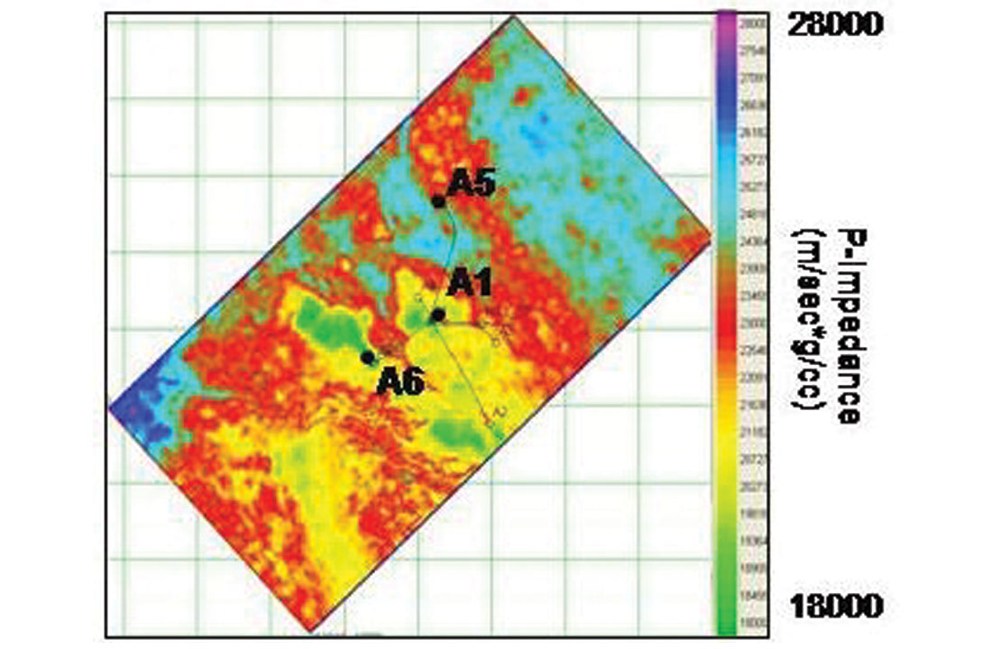
The model-based inversion result for the Marlin field is shown in Figure 4. In this figure, notice that there is differentiation between the gas and non-gas zones, but the wet well is still somewhat anomalous. However, the wells east of the A1 location are sitting on the edge of the seismic anomaly and may become better discriminated by utilizing the prestack information in the inversion process.

The AVO method

In the early 1980s, the AVO method was developed, in which the amplitudes of the seismic CMP gather as a function of angle were analyzed for hydrocarbon indicators. The equation that forms the foundation of AVO analysis has become known as the Aki-Richards equation (Aki and Richards, 2002). The original form of the equation can be re-formulated to give

where, A ,=

In equation (8), ΔV_P, ΔV_S, and Δρ indicate differences of the velocity or density across a layer boundary, and V_P, V_S, and ρ indicate averages of the velocity or density across a layer boundary. The A term is called the intercept and is a linearized version of the zero offset P-wave reflection coefficient given in equation (1). The B termed is called the gradient and the C term is called the curvature.

Standard AVO analysis involves using a least-squares fitting procedure to estimate A, B, and C from pre-stack seismic angle gathers and then cross-plotting B against A to identify deviations away from a wet trend line. The wet trend line can be derived by assuming that ρ and V_P are related by Gardner’s relationship (Gardner et al. 1974), given in linearized form by

and that V_S and V_P are related by Castagna’s equation (Castagna et al., 1985), given by

Alternately, the product of A and B will often reveal class 3 gas sands, in which the acoustic impedance of the sand is less that the surrounding sediments. Applying this method to the Marlin field gives the result shown in Figure 5(a). Note that the dry hole (A5) is now showing a negative AxB, or wet, signature. However, the wells east of A1 are also exhibiting a wet response.

The Aki-Richards equation was re-formulated by Fatti et al. (1994) as a function of zero-offset P-wave reflectivity R_P0, zero-offset S-wave reflectivity R_S0 and density reflectivity R_D in the form

where, c₁=1+tan²θ, c₂=–8ϒ²+tan²θ, ϒ=V_S/ V_P, and c₃=–0.5tan²θ+2ϒ² sin²θ, R_P0 is equivalent to the A term in equation (8), and the other two reflectivity terms are given by

Based on equation (11), Fatti et al. (1994) showed that a least-squares procedure could be implemented to extract the three reflectivity terms from the pre-stack seismic data. Using the extracted reflectivities R_P0 and R_P0 from this approach, the authors then modified the fluid factor approach (which had earlier been proposed by Smith and Gidlow (1987) is a slightly simpler form), which can be written:

The result of applying the fluid factor method to the Marlin field is shown in Figure 5(b). Note that the non-gas well (A5) is more anomalous than we saw in the previous figure, indicating that the fluid factor technique is inadequate for distinguishing fluids in this reservoir setting.

In the next section, we will show how to combine the techniques of model-based inversion and AVO to develop a technique that we will refer to as simultaneous inversion.

Pre-stack simultaneous inversion

As we have discussed, the goal of seismic inversion is to obtain reliable estimates of P-wave velocity (V_P), S-wave velocity (V_S), and density (ρ) from which to predict the fluid and lithology properties of the subsurface of the earth. This problem has been discussed by several authors. Simmons and Backus (1996) developed a scheme to invert for P-reflectivity (R_P), S-reflectivity (R_S) and density reflectivity (R_D) that was based on three assumptions: that the reflectivity terms can be estimated from the angle dependent reflectivity R_PP(θ) by the Aki-Richards linearized approximation, that ρ and V_P are related by Gardner’s relationship given by equation (5) and that V_S and V_P are related by Castagna’s equation of equation (6).

Buland and Omre (2003) use a similar approach which they called Bayesian linearized AVO inversion. Unlike Simmons and Backus (1996), their method is parameterized by the three terms, ΔV_P/V_P , ΔV_S/V_S , and Δρ/ρ., again using the Aki-Richards approximation. The authors also use the small reflectivity approximation to relate these parameter changes to the original parameter itself, as given in equation (4). Similar terms are given for changes in both S-wave velocity and density. This logarithmic approximation allows Buland and Omre (2003) to invert for velocity and density, rather than reflectivity, as in the case of Simmons and Backus (1996).

Hampson et al. (2005) extended the work of both Simmons and Backus (2003) and Buland and Omre (1996), and developed a new approach that allows us to invert directly for P-impedance, S-impedance, and density. It was also the goal of this work to extend model-based post-stack impedance inversion method so that this method could be seen as a generalization to pre-stack inversion. To do this, equation (4) can be combined with equation (11) to give

where L_S = ln(Z S) and L_D = ln(ρ). Note that the wavelet is now dependent on angle.

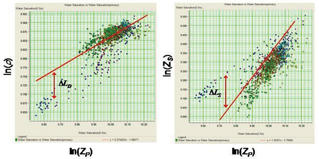
Equation (13) could be used for inversion, except that it ignores the fact that there is a relationship between L_P and L_S and between L_P and L_D. Because we are dealing with impedance rather than velocity, and have taken logarithms, the relationships are given

and

That is, we are looking for deviations away from a linear fit in logarithmic space. This is illustrated in Figure 6.

Combining equations (14) through (15), we get

where

Equation (16) can be implemented in matrix form as

If equation (17) is solved by matrix inversion methods, we again run into the problem that the low frequency content cannot be resolved. A practical approach is to initialize the solution to, [L_P ΔL_S ΔL _D]^T = [In(Z_P0) 0 0]^T where Z_P0 is the initial impedance model, and then to iterate towards a solution using the conjugate gradient method.

Model Example

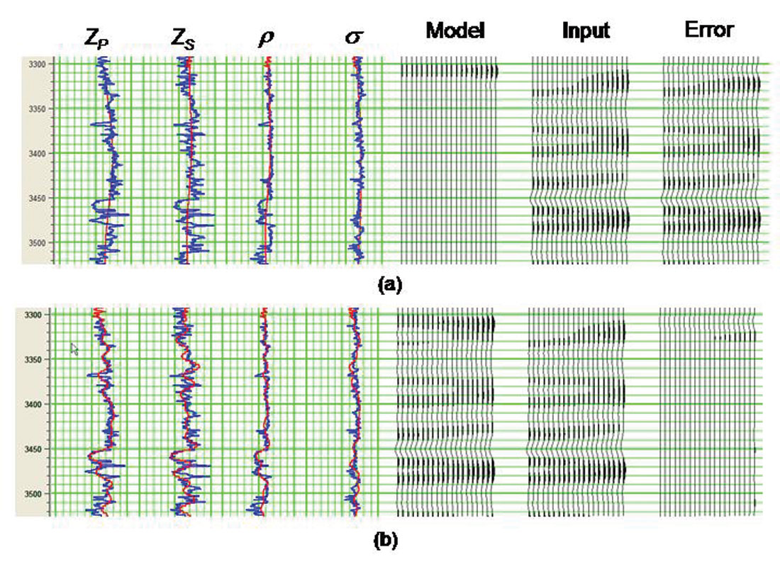
We will now apply this method to a model data example. Figure 7(a) shows the well log curves for a gas sand on the left (in blue), with the initial guess curves (in red) set to be extremely smooth so as not to bias the solution. On the right are the model, the input computed gather from the full well log curves, and the error, which is almost identical to the input. Figure 7(b) then shows the same displays after 20 iterations through the conjugate gradient inversion process. Note that the final estimates of the well log curves match the initial curves quite well for the P-impedance, Z_P, S-impedance, Z_S, and the Poisson’s ratio (σ). The density (ρ) shows some “overshoot” above the gas sand (at 3450 ms), but agrees with the correct result within the gas sand. This is most likely attributable to the fact that NMO-stretch has not been included in the model. The results on the right of Figure 7(b) show that the error is now very small.

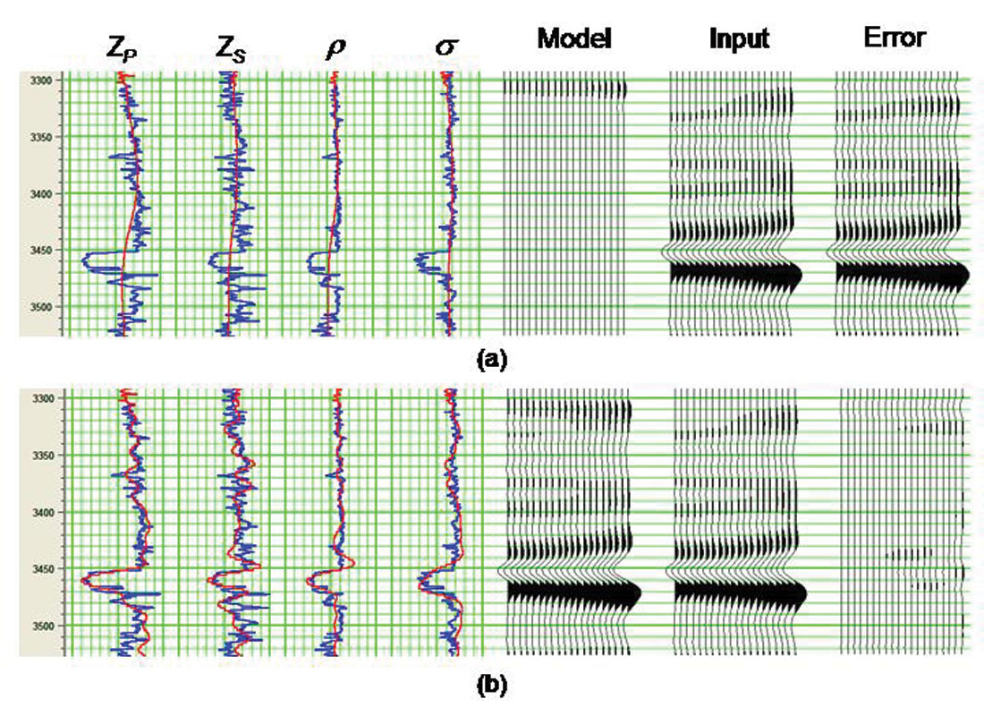
Next, we will use Biot-Gassmann substitution to create the equivalent wet model for the sand shown in Figure 8, and again perform inversion. Figure 8(a) shows the well log curves for the wet sand on the left, with the smooth initial guess curves superimposed in red. On the right are the model from the initial guess, the input modeled gather from the full well log curves, and the error. Figure 8(b) then shows the same displays after 20 iterations through the conjugate gradient inversion process. As in the gas case, the final estimates of the well log curves match the initial curves quite well, especially for the P-impedance, ZP, S-impedance, ZS, and the Poisson’s ratio (s). The density (r) shows a much better fit for the wet sand (which is at 3450 ms) than it did for the gas sand.

It is important to point out that, while these results are very good, the quality of the data that went into the study was also very good. For example, we used an angle range from 0 to 60 degrees, which is higher than found in most seismic surveys. Also, the data was synthetic and thus noise-free. In the next section, we will therefore apply this method to real data and see how well it performs.

Real Data Example

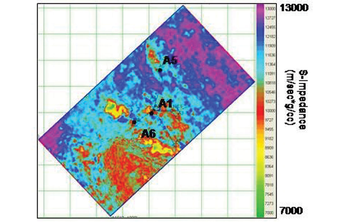
Next, we will return to the Marlin field and apply the simultaneous inversion approach to this dataset. Recall that the P-impedance inversion was shown in Figure 4. However, we noted earlier that this P-impedance inversion result is ambiguous in terms of differentiating fluid effects from lithologic or porosity effects, and we need S-impedance and density to get a better estimate of these parameters. The advantage of simultaneous inversion is that S-impedance and density are produced along with the P-impedance. The S-impedance inversion for the Marlin field is shown in Figure 9. Note that, although the three wells are still located on anomalous regions, the S-impedance trends are quite different from the P-impedance trends shown in Figure 4.

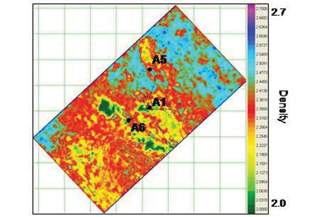
The density inversion for the Marlin field is shown in Figure 10. Again, note that the three wells are located on anomalous regions of density but that the trends are different from the P-impedance trends shown in Figure 4. Although all three wells are associated with density anomalies, this is most likely due to sand presence with the larger drops in density being influenced by gas.

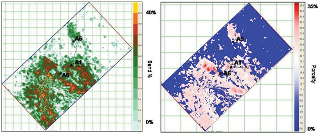
Finally, we will use the output of the simultaneous inversion to predict fundamental properties of the reservoir such as porosity, sand percentage, and water saturation.

For the sand shale separation and porosity transformation, this will be done empirically by calibration to the well data. Figure 11(a) shows a cross-plot of density versus Vshale for the three wells shown on our earlier figures (A1, A5 and A6). As shown by the picked zones in this cross-plot, we were able to separate sand from shale using a cutoff of 2.32 g/cc, where sands are lower density and shales higher. The slightly transparent rectangular polygons of blue and gold, respectively, represent shales with higher quartz content and sands that have higher clay content. The result of this transformation to sand and shale is shown in Figure 12(a), where the values represent sand frequency or a simplified net-to-gross.

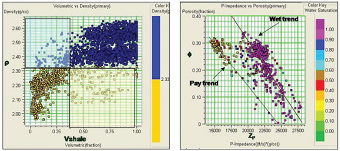
Figure 11(b) shows a cross-plot of porosity versus P-impedance for the three wells A1, A5 and A6. As shown by the lines of this cross-plot, we can derive two empirical formulas for porosity from the inverted P-impedance volume. We again use a cutoff to separate pay from non-pay (18,000 ft/sec*g/cc), then an empirical relationship is defined for pay and non-pay. The result of this transformation to porosity is shown in Figure 12(b). The average porosities from the well log data is about 27%, which is closely supported by the seismic derived porosities.

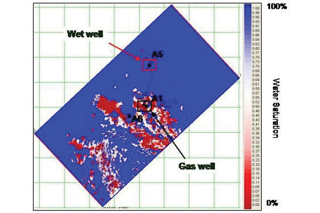
Now that we have derived the porosities over the Marlin field, we can transform to water saturation using the porosity cube and the density cube. This involves transforming the relationship between saturated density, water saturation, and porosity, given by

to an equation in which water saturation is on the left hand side of the equation, given by:

In equation (19) we let ρ_gas = 0.1 ρ_W = 1, and ρ_matrix =2.65.

The result of this transformation is shown in Figure 13, which is the water saturation map at the zone of interest. Notice that the A5 well is shown as 100% water saturated, and that the A1 and A6 wells are shown as gas producers, which are the correct results, as well as the wells to the east of the A1 well.

Conclusions

In this tutorial, we have discussed the history of seismic amplitude inversion, from its origin as a post-stack process to the most recent developments which involves the simultaneous inversion of pre-stack seismic data. Although post-stack inversion is a powerful and robust method, it suffers from the fact that its final product, P-impedance does not allow us to discriminate between lithology, porosity and fluid effects. Other limitations of poststack inversion, such as its inability to recover the low frequency components of the impedance, and the effects of seismic noise and scaling problems, are inherent limitations of the seismic data itself. These data limitations lead to the development of new seismic processing algorithms and new approaches to the technique of inversion, such as model-based inversion.

The inability of post-stack inversion to discriminate between the lithology and fluid content of the reservoir lead to the development of the AVO technique for the analysis of pre-stack data. We briefly reviewed the AVO method and then showed that the theory of AVO could be coupled with the traditional approaches of post-stack inversion to produce estimates of P-impedance, S-impedance and density. The simultaneous inversion method that we discussed is based on three assumptions: that the linearized approximation for reflectivity holds, that reflectivity as a function of angle can be given by the Aki-Richards equations, and that there is a linear relationship between the logarithm of P-impedance and both S-impedance and density. We illustrated our inversion methods using modelled gas and wet sands and also a real seismic example which consisted of a gas sand play from the Gulf of Mexico. In our real data example, we showed that the extraction of the primary attributes of P and S-impedance and density from our seismic data allows us to directly predict porosity, sand percentage and water saturation. These predictions correlated extremely well with known results.