An introduction to common offset vector trace gathering

Summary

This paper is an introductory review of the recently developed concept of common offset vector (COV) trace gathering. The COV trace gathering is a 3D generalization of conventional 2D offset gathering. A COV gather is a similar but different representation of a common-offset common azimuth gather. For many types of acquisition geometry with regular sampling, a COV gather should be a single-fold trace gather with a survey-size continuous coverage. The COV gathering can also be described as a tile-connection scheme from the cross-spreads in a 3D geometry. The COV gathering parameters are determined by acquisition parameters. The COV gathers can be useful in many aspects of processing prestack 3D seismic data, especially for the analysis of azimuthally varying data attributes.

Introduction: offset gathering of 2D data

An offset gather refers to a group of prestack traces with a limited range of offsets. The term “common offset gather” is often used for such trace gathers, even though the offsets within a gather do not have to be the same. I call an offset gather “valid” if it has a continuous CDP coverage of the size of the whole survey, 2D or 3D. The word “continuous” is used in the sense that the pertinent data are sampled with the finest spatial rate of the survey, for example, the CDP bin size. The word “valid” is used in the sense that such a gather, by itself, provides a continuous full-range subsurface image.

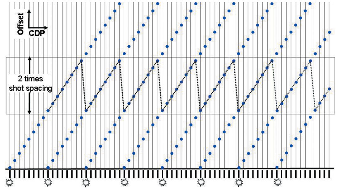
Grouping seismic data into offset gathers has been a routine procedure for velocity analysis, prestack imaging and prestack data interpretation, such as AVO analysis. This section reviews the routine calculations for forming offset gathers for 2D data. Figure 1 shows the stacking chart of a perfectly regular 2D acquisition geometry with one-sided spreads. An offset range of at least two times the shot interval is required to ensure a valid offset gather. In fact, because of the geometry regularity, an offset gather has one and only one trace at each CDP when its offset range is two times the shot interval. Such single-fold valid offset gathers have the highest possible offset resolution, besides the highest CDP resolution. They are desirable for producing high quality migration results for migration velocity analysis and AVO analysis. The offset range of an offset gather is often called the bin-size of the offset gather.

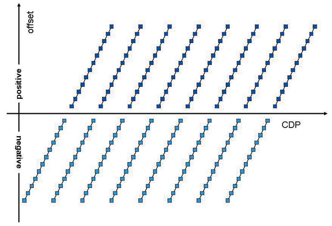
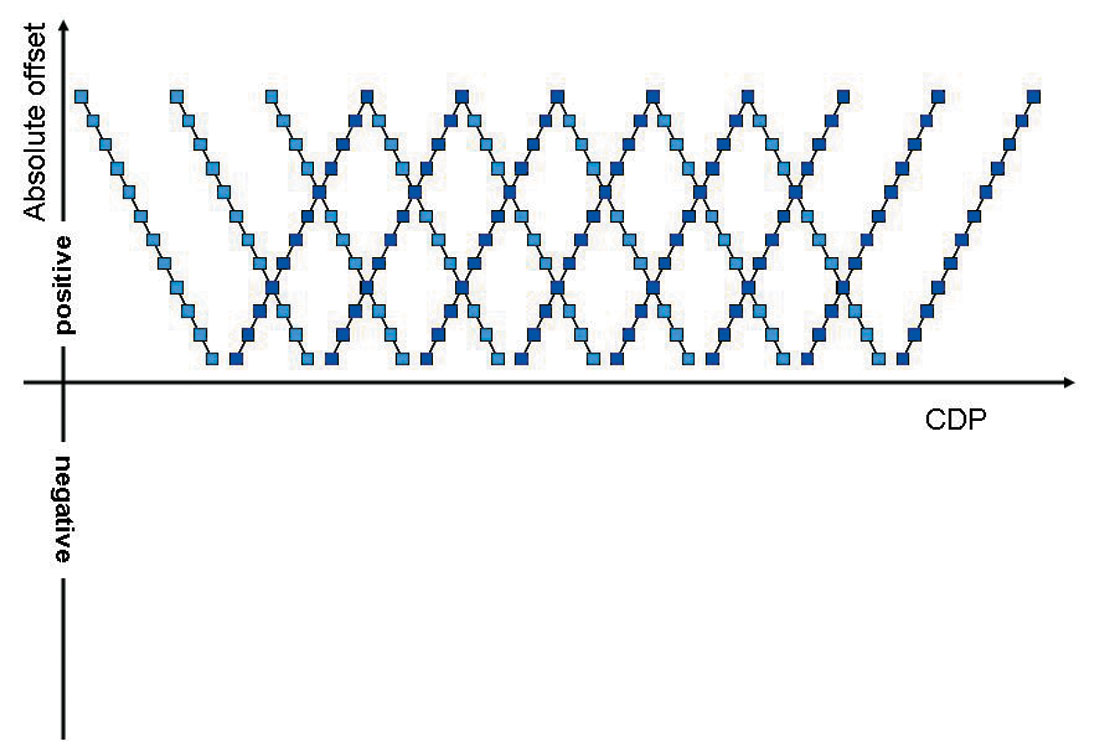
One-sided spread geometry describes conventional marine 2D seismic data acquisition. However, typical land 2D surveys use two-sided spreads, where active receivers are located on both sides of each source. Offset gathers for two-sided spreads can be formed by using signed offsets or by using absolute values of the offsets. When negative offset and positive offsets are gathered separately, an offset bin-size of two times the shot interval is required to ensure a valid offset gather, as in the one-sided spread case. However, when the absolute offset values are considered, offset bin-size of only one shot interval is enough to produce valid offset gathers, since the negative and positive offsets compensate each other by covering alternate CDP ranges (see Figure 2). The total number of single-fold valid offset gathers (non-overlapping) is always equal to the nominal fold of the survey.

The parameters to form 2D single-fold valid offset gathers are determined by the acquisition parameters: the source interval, receiver group intervals and the total offset range. The same scheme can be directly applied to 3D surveys with very narrow azimuth ranges, such as conventional towed streamer marine 3D surveys (with some ignorable difficulty at the very near offsets). However, things become more complicated with 3D land, wide azimuth surveys. Nowadays, prestack data processing for land 3D datasets has been mostly using conventional 2D approaches. The formation of offset gathers mostly ignores the implications of the azimuth dimension. This approach has found itself in a difficult situation when dealing with concerns regarding the number of offset gathers to form, the fold distributions of each offset gather, and azimuth variation within an offset gather. It is practically impossible, with this 2D approach, to form 3D offset gathers that are both single-fold and valid, even when the acquisition geometry is perfectly regular. This paper discusses the COV gathering scheme, which can form single-fold valid offset gathers (COV gathers) for regular wide azimuth surveys.

Common offset vector

The offset of a trace is defined as the distance between its source and its receiver. It ignores the directional property of a trace and becomes inappropriate when dealing with processing procedures such as the prestack migration and the interpretation of azimuthally varing attributes. A combination of offset and azimuth is commonly used to describe a 3D trace and has been successful in theoretical and practical aspects of 3D seismic data processing. This paper discusses a different representation of the directional distance between a trace’s source and receiver. A 3D survey geometry grid has an inline direction and a crossline direction (We assume that the inlines are parallel to the receiver lines). The source-receiver offset, as a vector, can be projected onto these two directions and represented by two scalar offset values, called inline offset and crossline offset. This pair of scalars represents an offset vector in Cartesian coordinates, in contrast to the offset-azimuth representation in polar coordinates. It is intuitively advantageous to use the Cartesian representation because 3D data are acquired in rectangular (possibly skewed), not circular, spreads.

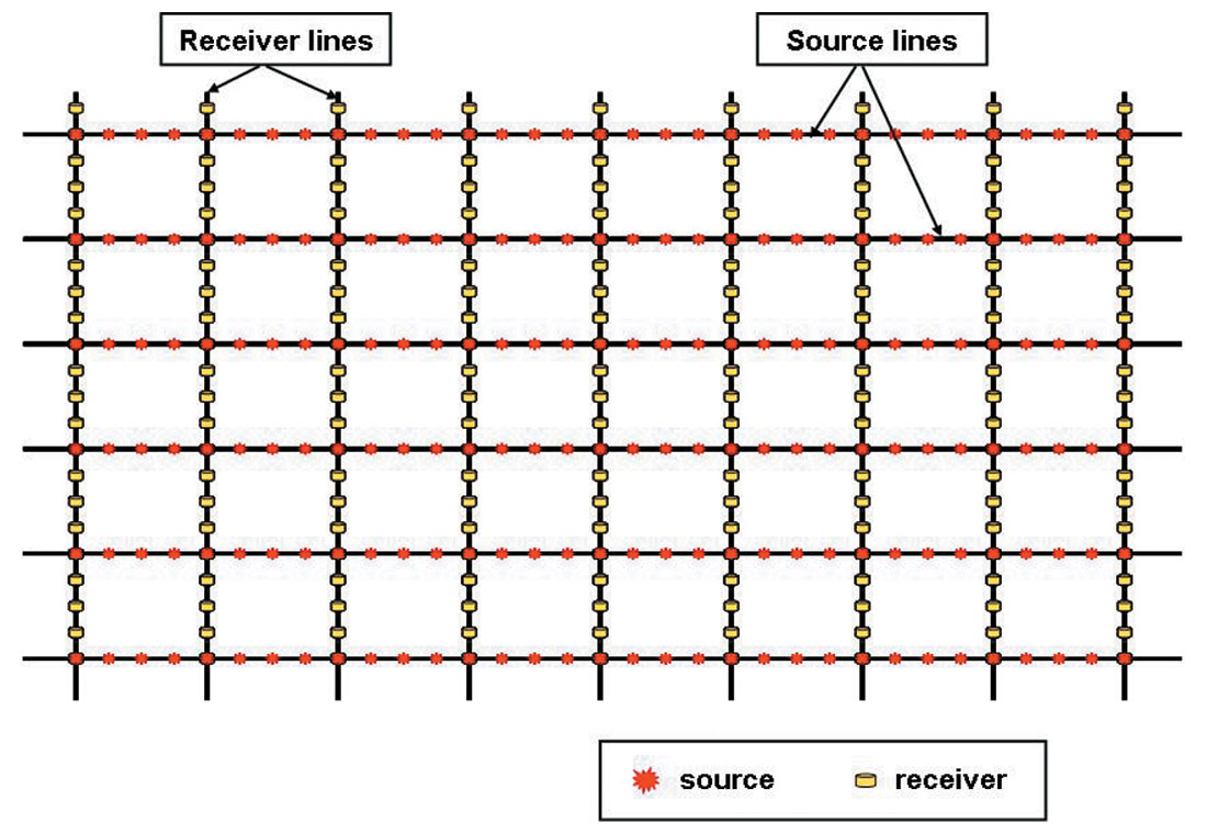
The next few sections consider, if not otherwise indicated, a regular, perpendicular 3D survey as partly shown in Figure 3. This survey has equally spaced receiver lines and equally spaced source lines, and these two spacings can be different. The receivers on each receiver line are evenly spaced, and this spacing is the same for all the receiver lines. The sources on each source line are equally spaced and this spacing is the same for all the source lines. All receivers active for one source form a patch for the source. The regular geometry in consideration assumes a uniform patch size for all the sources. To be more specific, we assume that the patch size is 12 receiver line spacings wide and 10 source line spacings long. Every source is always located closest to the geometric center of its patch.

A 3D bin line as collection of 2D lines

Let’s start with one CDP bin inline in the survey, shown in Figure 4 as a dotted line. The receiver and source locations of traces on this line are limited by the size of the source patches. If a trace belongs to a CDP on this line, its receiver has to be on the receiver lines A to F, and its source has to be one of the sources whose lateral locations are indicated by the numbers 1 to 6. More precisely, if its source is one of the sources at lateral location 1, then its receiver must be from the receiver line marked by A. Similarly, if the source is at location 2, the receiver must be on receiver line B; the relations between 3 and C, 4 and D, 5 and E, 6 and F are the same. All the traces on this CDP line are thus grouped into six 2D CDP lines that can be identified with fixed source - receiver pairs, namely 1 A, 2 B, 3 C, 4 D, 5 E, and 6 F, respectively.

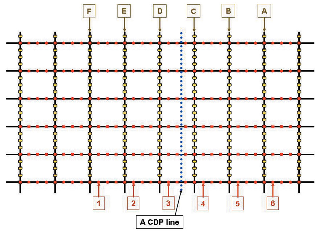
For traces on each of these 2D lines, their sources are along a line parallel to the receiver line, but possibly with a distance between them. This is to say that these traces have the same crossline offset. If we ignore the crossline offset, the traces’ inline-offsets and CDP locations construct a 2D regular stacking chart as shown in Figure 2. Note that the source spacing of these six 2D lines is the same, and it is the source line interval for the 3D geometry. Therefore, by using two times the source line spacing as the offset bin-size, each of the six 2D lines forms single-fold valid offset gathers. The combination of these 2D inline-offset gathers becomes a six-fold valid offset gather for the 3D CDP line in consideration. This obviously is not our ultimate result. However, by the definition of the inline-offset and crossline offset, and the geometric reciprocity of the source and receiver we should be able to further the offset gathering process using crossline-offset variations.

Now let’s consider a CDP bin crossline parallel to the source lines. This 3D bin line can also be decomposed into a number of 2D lines. On each of these 2D lines, a number of 2D single-fold valid offset gathers can be formed using crossline offset values, and the offset bin-size should be twice the receiver line interval.

Finally, by combining these two 2D offset gathering schemes, we can construct a 3D scheme, the COV scheme, to form 3D singlefold valid offset gathers. Any given trace in the geometry belongs to an inline and a crossline. It also has an inline offset and a crossline offset. As an inline trace, its inline offset, with other acquisition parameters, determines which single-fold valid inline-offset gather it belongs to; as a crossline trace, its crossline offset is used to determine which crossline-offset gather it belongs to. This is to say that a trace’s inline offset and crossline offset determine which single-fold valid offset vector gather it belongs to. Such a single-fold valid offset vector gather is called a COV gather. The total number of COV gathers is determined by the number of single-fold valid gathers in both inline and crossline directions. The single-fold property and the full coverage property of a COV gather come from these properties of the two 2D offset gathering schemes. The number of COVs for a 3D survey should equal the survey’s nominal fold.

COV gather as connected tiles from cross-spreads

A COV gather can also be formed equivalently based on the concept of cross-spreads. A cross-spread is defined as all the traces with their sources on same source line and their receivers on same receiver line. Across-spread in a fairly regular geometry is single-fold and it has continuous subsurface coverage (in the sense of minimum spatial sampling intervals in both directions of a survey grid). The CDP coverage of a cross-spread is practically the same as the coverage of the center shot record (the source closest to the receiver line of the cross-spread). In the present example geometry, the size of the CDP coverage of a cross-spread can only extend up to three receiver lines on each side of the receiver line of the cross-spread and two and a half source line spacings on each side of the source line of the cross-spread, as shown in Figure 5.

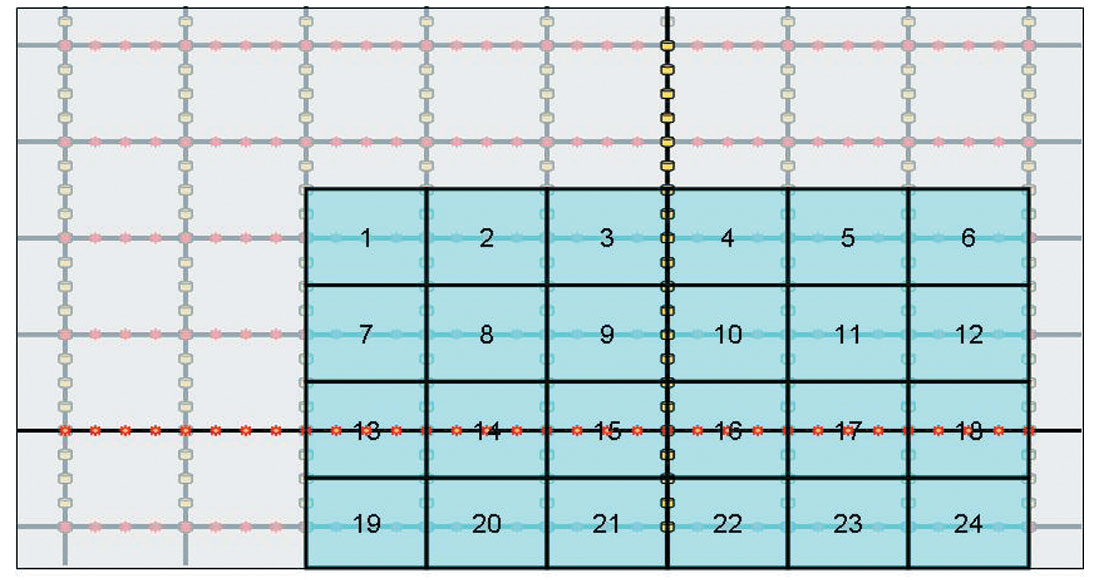
Besides numerous advantages, cross-spreads have some drawbacks. They have very limited coverage are a , practically unlimited offset range (usually the maximum range in the survey), and unlimited azimuth range (usually full 360 degrees). The large offset range prevents them from being used for velocity analysis and AVO analysis. Their small coverage areas limit their application in migration processes. The COV gathering was introduced here as a solution to create full-coverage, limited offset and limited azimuth gathers by “patching” together parts of different cross- spreads (Vermeer 1998). The region between two adjacent source lines and two adjacent receiver lines in a cross-spread is called a tile. As shown in Figure 5, a cross-spread can be sectioned into little areas and each of them has the size of a typical tile. These sections can cross the source line and the receiver line if necessary. We develop a systematic indexing scheme based on the sections’ relative positions to the zero-offset location (center) of the cross-spread (Figure 5). We apply the indexing to all the cross-spreads. It can be verified that two sections from two neighbouring cross-spreads but with the same index number connect to each other without either overlap or gap. Therefore all the sections with the same index number form a single-fold full-coverage of the survey. Each one group of the same numbered sections is a COV gather.

Practical complications

Determination of the COV parameters

From the discussions above, we can extract a practical approach to form COV gathers. For inline offsets, the offset bin-size of a COV should be twice the source-line spacing because it is equivalent to the source interval on a 2D line parallel to the receiver lines. Similarly, the offset bin-size for crossline offsets of a COV should be twice the receiver line spacing. The minimum and maximum of signed inline offsets and crossline offsets can be determined by the size of the typical source patch of the survey.

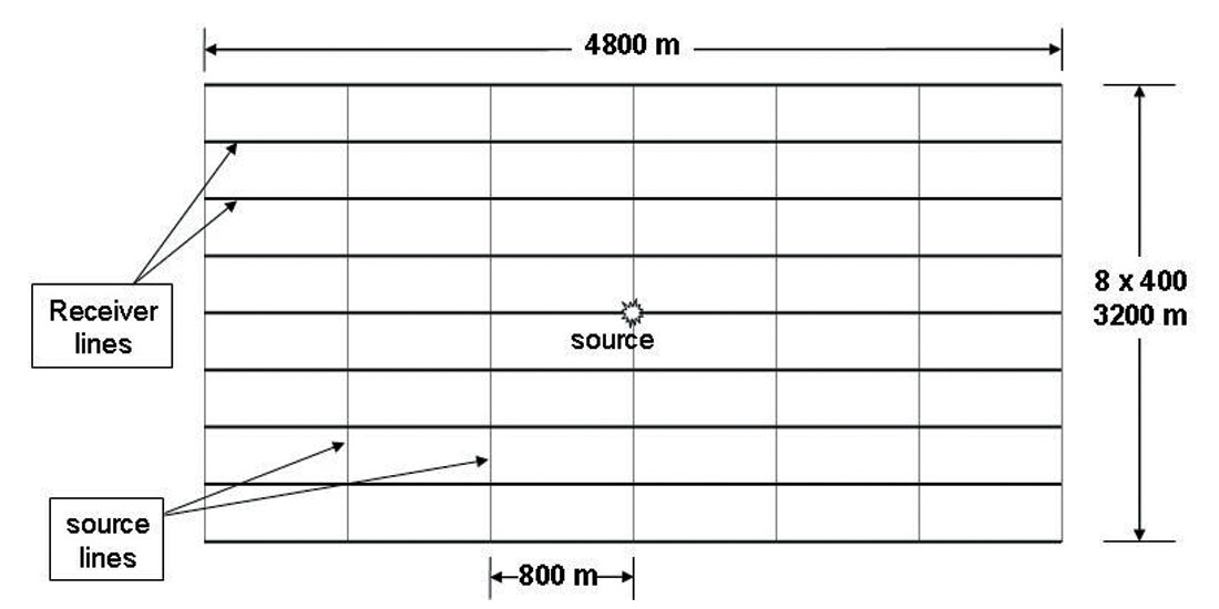
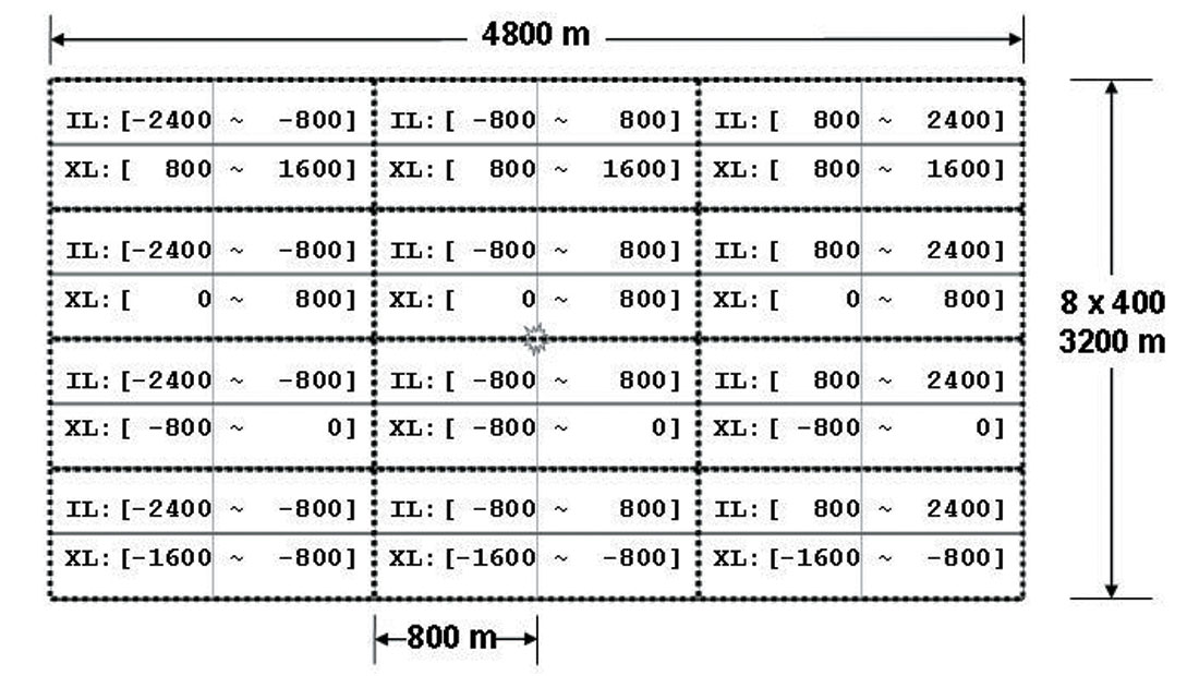
Let’s go through the COV gathering procedure with an example. Figure 6 shows a patch with inline dimension of 4800 meters and crossline dimension of 3200 meters. The source line spacing is 800 meters and the receiver line spacing is 400 meters. There are 6 x 8 = 48 tiles in the patch. The fold of this 3D survey should be 12, and we should have 12 COV gathers formed. Since the source is located at the geometric center of its patch, the minimum inline offset is -2400 meters and the maximum inline offset is 2400 meters; the minimum and maximum crossline offsets are -1600 meters and 1600 meters, respectively. Using inline-offset bin-size of 2 x 800 = 1600 meters and three center locations of -1600 m, 0 m, and 1600 m, the total range of -2400 to 2400 meters is covered. Similarly, using crossline-offset bin-size of 2 x 400 = 800 meters and four center locations of -1200 m, -400 m, 400 m, and 1200 m, the range of -1600 to 1600 meters are covered. The total number of centers will be 3 x 4 = 12. Figure 7 shows the COV gathers with their corresponding rangs in inline offsets and crossline offsets.

The offset range of a COV gather

The offset ranges within each COV gather are remarkably larger than that we are usually familiar with. In the example in Figure 7, the largest offset difference can be as large as 1750 meters at the corner COVs (from 1131 m to 2884 m). Such large offset range within a COV gather is not desirable, and is probably one of the reasons why the COV gathering has not been widely used in routine data processing. Let’s put this offset range issue into perspective. In more realistic cases, the fold coverage of land 3D surveys is much higher than 12, ranging from around 30 to several hundreds. Offset range within a COV is accordingly much smaller. Also, the COV gathering attempts to sample both the offset dimension and the azimuth dimension at the same time. The reduction of offset sampling density is expected to be compensated by denser sampling in azimuth dimension. In the example shown in Figure 7, the 12 COVs represent 10 different azimuth values within the 360 degree range. Furthermore, when source-receiver reciprocity is assumed, two COVs from two opposite direction and same offset range can be combined to create two new COVs with much smaller offset ranges. Herrmann et al (2007) discovered this combination method and they call these new COVs “high resolution (HR)” because of denser offset sampling. Vermeer (2007) also gives some discussion on this topic. In the present example, a corner COV, for example (IL: [800~2400], XL: [800~1600]), along with its opposite COV, (IL: [-2400~-800], XL: [-1600~-800]), produces two new HR COVs with offset range of about 1131~2530 meters and about 1789~2884 meters respectively. This innovative application of the reciprocity is similar in principle to the offset coverage compensation in the 2D two-sided spread acquisition shown in Figure 2.

Perpendicularity not essential

All the discussions so far are dealing with perpendicular source lines and receiver lines, but the perpendicularity is not essential to the COV concept. If the source lines and receiver lines are not perpendicular to each other, the shape of the coverage of cross-spreads will be a parallelogram rather than the rectangular shape described above. A similar sectioning and numbering scheme can be applied to these parallelogram-shaped cross-spreads and COVs can thus be formed accordingly from these parallelogram-shaped tiles.

Another option is to calculate the effective source distance parallel to the receiver lines and the effective source distance perpendicular to the receiver lines. The new source distances can then be used to form “rectangular” COVs. These effective source distances are not uncommon in 3D processing; geophysicists are using a similar concept when they calculate the CDP bin-size when constructing geometry bin grids (which are always rectangular). Conventional marine 3D geometry is an extreme case, where the source lines are parallel to the receiver lines. When the azimuth is so limited that it is often ignored in the processing sequence, the COV concept seems unnecessary. However, the inline offset and crossline offset concepts can still be useful. For example, when forming offset gathers, the crossline offsets can be ignored and the channel numbers can be effectively used as inline offsets. Using channel numbers instead of source-receiver offsets can put all near-gun channels from all the streamers into one offset gather. Even though the offset range of these near-gun gathers can be “too large”, the continuity of the CDP coverage may improve the migration quality of near offset gathers.

Geometry irregularity

Acquisition geometry irregularity does not cause problems specific to COV gathering. On the other hand, COV gathers can handle irregularity better than conventional offset gathering in many aspects. The conventional offset gathering method practically ignores the acquisition geometry, whether it is regular or not. It is impossible to form offset gathers with even fold distribution by simply gathering traces using only the source-receiver offsets, because the distribution of fold along offsets is always irregular for wide-azimuth 3D geometries.

Any CDP binning grid has a certain size; a slight deviation from perfectly regular positioning usually does not move a trace from one CDP to another. This also means that slight mis-positioning of a trace (source and receiver locations) does not cause any problem in producing single-fold valid off s e t gathers. When acquisition irregularities necessitate borrowing or interpolating traces for the missing locations, the COV gathers need less effort in such regularization processes.

Possible applications

The COV gathers can be very useful when both azimuth and offset information has to be kept after migration. The COV gathering couple the azimuth and offset binning naturally, and this is different from the conventional azimuth sectoring plus a separated offset gathering. The difficulties of creating offset gathers with even fold distributions will only be more serious after azimuth sectoring. Amplitude variation with offset and azimuth (AVAz) and velocity azimuthal variation are two examples of such azimuthally variant attributes where COV gathering can provide help.

In many implementations of prestack migration of 3D land data the large trace density variation with offset becomes a concern. The number of traces in the middle offset range is many times more than the near offset and far offset ranges. By forcibly producing even-spaced offset sampling, middle offset traces have to be weighted down. However, once the even-spaced offset sampling requirement is removed, more reasonable approaches for prestack trace gathering are possible. Wilkinson (2007) uses flexed offset binning to prepare offset gathers for migration that is able to preserve the trace density variation after migration. Migration of individual COV gathers automatically preserve both offset and azimuth information. The offset sampling is somewhat compromised due to better azimuth sampling. These approaches tend to give all input traces the same weight, at least with fairly regular geometries. This is intuitively more desirable since it is difficult to find convincing reasons for preferring some traces over others. Especially since the preferred traces tend to be at the noisy near and far offsets.

Conclusions

The COV concept has been around for 10 years. It was first introduced by Vermeer (1998) and Cary (1999) from different viewpoints (under different names). This paper has reviewed the concept of COV gathering from both the 2D offset gathering concept (Cary, 1999) and the cross-spread concept (Vermeer, 3D cross-spread acquisition creates irregularities in offset gathers even when the acquisition geometry is perfectly regular. The COV gathering process clears up some confusing issues in forming single-fold, large coverage, limited offset, limited azimuth gathers. The acquisition parameters fully determine how the COV gathers are formed. The COV gathering is yet to be widely used in the industry. One reason is probably the large offset range within each COVs. Herrmann et al. (2007) has found a way to significantly improve the offset sampling of COV gathers using source-receiver reciprocity. I believe COV gathering is useful in many aspects of 3D wide-azimuth data processing.

Acknowledgements

I thank my employer, CGGVeritas, for granting the permission to publish this paper. I also thank many of my colleagues who have given helpful suggestions and comments.