Amplitude-vs-Offset and Seismic Rock Property Analysis: A Primer

Introduction

In this article, we’ll examine the basics of amplitude variations with offset (AVO) and rock properties derived from them. First we’ll look at the physical cause for AVO behavior. We’ll then discuss the quantitative methodologies for calculating attributes which describe the AVO behavior of pre-stack seismic data. At the same time, we’ll show methods of interpreting these attributes and how they can help to differentiate between regional geology and hydrocarbon reservoirs. We will then move on to extensions of AVO analysis that actually estimate elastic properties of the rock layers.

Note that we are not addressing seasoned AVO and seismic rock property interpreters, but those geophysicists, geologists, technicians and so on who still haven’t been exposed to the theory and practice but would like to know more about these methods.

In the end, what we would like you to get from this paper is the idea that changes in seismic amplitude with offset (AVO affects) are due to contrasts in the physical properties of rocks. Going further, quantitative analysis of AVO effects can yield attributes that discriminate between different lithologies and fluids. Finally, further analysis can lead directly to estimates of the elastic properties that gave rise to the AVO effects in the first place and help lessen the uncertainties of interpretation.

Amplitude Variation with Offset: Seismic Energy partitioning at boundaries

Amplitude variation with offset comes about from something called ‘energy partitioning’. When seismic waves hit a boundary, part of the energy is reflected while part is transmitted. If the angle of incidence is not zero, P wave energy is partitioned further into reflected and transmitted P and S components. The amplitudes of the reflected and transmitted energy depend on the contrast in physical properties across the boundary. For us seismic people, the important physical properties in question are compressional wave velocity (Vp), shear wave velocity (Vs) and density (ρ). But, the important thing to note is that reflection amplitudes also depend on the angle-of-incidence of the original ray (Figure 1).

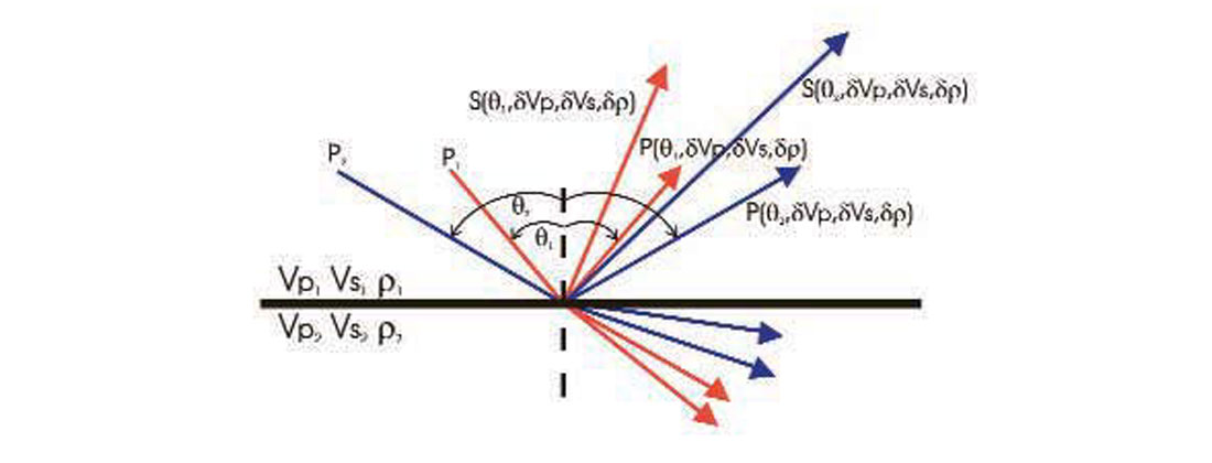
So if we know how the amplitudes of a reflector from a CDP change with angle-of-incidence, we can figure out something about how the physical properties of the rocks are changing across the boundary. How amplitudes change with angle-of-incidence for elastic materials is described by the quite complicated ‘Zoeppritz equations’ (as well as higher-level approximations like that of Aki and Richards in their famous seismology textbook of 1979). But there are many different simplifications of these equations that make analysis of amplitudes with angle much easier.

One thing to point out now is that ‘amplitude variation with offset’ is not always an appropriate term. For proper analysis, we need to examine ‘amplitude variation with angle’.

Mechanics of quantitative AVO analysis

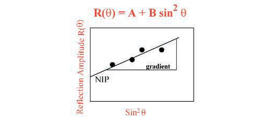
Quantitative AVO analyses are done on common-midpoint-gathers (or super-gathers, or common-offset gathers, or as they’re called in the AVO business ‘Ostrander gathers’ – see Ostrander, 1984). At each time sample amplitude values from every offset in the gather are curve-fit to a simplified, linear AVO relationship (Figure 2). A better way of saying this is that we fit a best-fit straight line to a plot of amplitude versus some function of the angle of incidence. This yields two AVO attributes - basically the slope and intercept of a straight line - which describes, in simpler terms, how the amplitude behaves with angle of incidence.

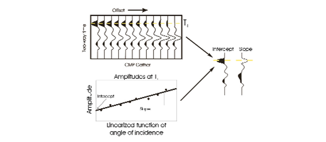
There are a lot of equations that have been used over the last 15 years or so, but all of them, no matter what interpretation is given to the ‘intercept’ and ‘slope’, work in this same way.

AVO necessities

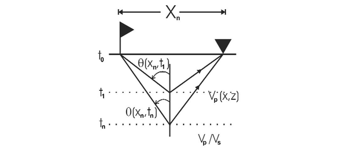
To use these AVO approximations for quantitative analysis, there are a few necessary inputs. First, we need a P velocity model to calculate a relationship between offset, travel-time and angle-of-incidence (Figure 3). Secondly, we need a Vp/Vs background constraint since usually one of the assumptions made is that we know this (see the ‘B’ term in Shuey’s Equation in Figure 5, for instance). Finally, we need offsets that give enough angles-of-incidence for an accurate fitting of the straight line (in practice, somewhere around at least 22 degrees).

Example data set

In order to examine a couple of the methodologies available for quantitative AVO analysis, we’ll use a model that was constructed from real well logs from the western Canada basin (Figure 4). In this example we have Bluesky and Halfway gas sand reservoirs. There are two things to note about AVO and this data set. First, though the seismic response is synthesized, the physical properties, as measured in well-bores, are real and so then are the AVO responses. Second, even though the examples are clastic gas reservoirs, the basic concepts can be applied to many different lithologies and reservoir types including carbonates.

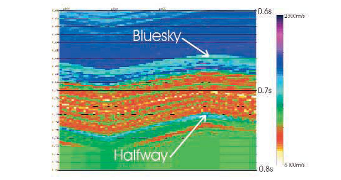
The Bluesky gas sand is higher impedance than the encasing shales (this is a Class I anomaly in the classification scheme of Rutherford and others, 1989). This means that on gathers, we would see a peak which dims with offset.

The Halfway gas sand is lower impedance than the encasing evaporites and carbonates (a Class III AVO anomaly). This means that we see a trough that increases in amplitude with offset on gathers. This is the classic “bright spot” anomaly we’ve all heard of.

Shuey Equation

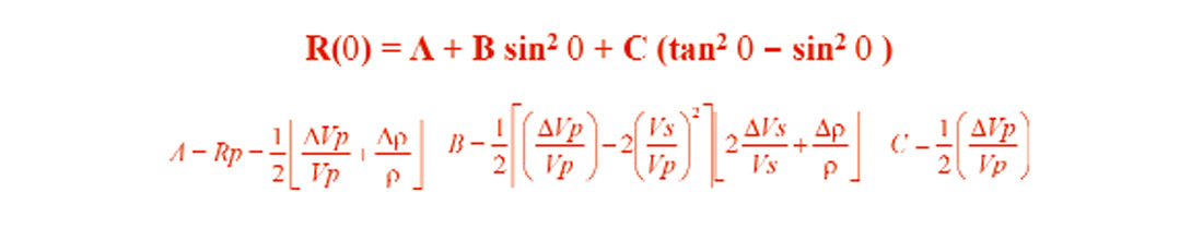
Shuey (1985) came up with a simplification to the complicated AVO Zoeppritz Equation (actually, he used the Aki and Richards approximation to Zoeppritz). The equation shown (Figure 5) has three terms. But if we ignore the “C” part, we are left with a linear equation (the familiar ‘y=mx+b’ from high school math). This equation does not handle high angles of incidence well, but it is simple to understand and is still very much in use today. What’s done is that the amplitudes at every time sample of an NMO’d gather are plotted against the squared sine of the angle-of-incidence (Figure 6). The intercept describes the “normal-incidence P-reflectivity” (NIP) while the slope is the gradient (how the amplitude changes with angle).

It’s worth repeating that all current quantitative AVO methods work this way. That is, amplitude changes are fit to a linear (i.e. two term) AVO approximation from which two attributes can be extracted. These two attributes describe the AVO character of the pre-stack gathers. The only difference with the various methods is in the complexity and accuracy of the approximation used and what two particular AVO attributes can be pulled out.

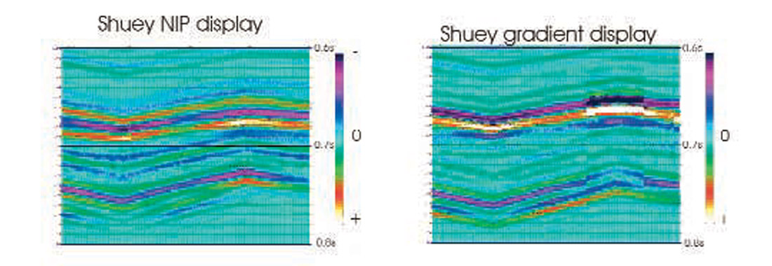
We show the Shuey NIP and gradient display in Figure 7. The NIP is simply an estimate of the normal incidence reflectivity while the gradient indicates whether the amplitude is increasing or decreasing with offset and how strongly. Though these two attributes can be combined (along with other assumptions) to create other attributes, more sophisticated methods yield more useful and interesting attributes.

Fatti Methodology

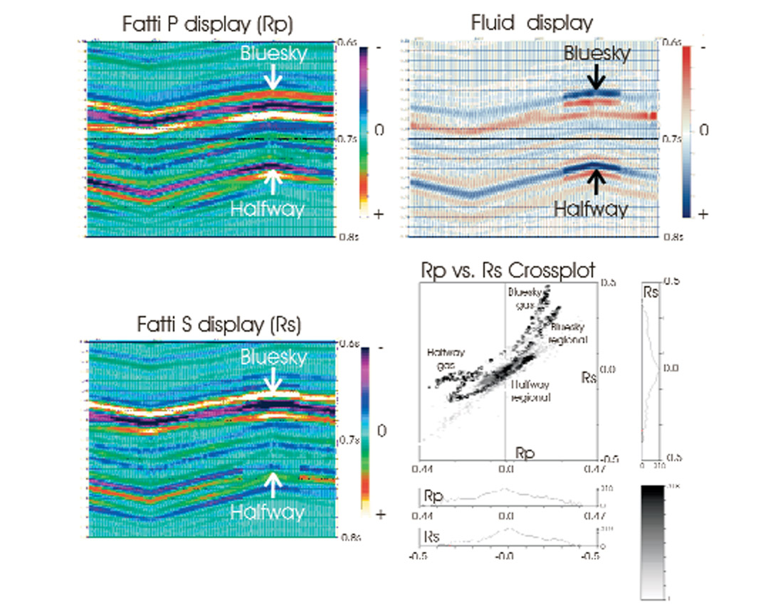
The Fatti methodology (Fatti and others, 1994) is a much more sophisticated AVO approximation than Shuey’s (Figure 8). This methodology not only is more accurate to higher angles-of-incidence, but is independent of any assumption of density and allows any meaningful Vp/Vs as a constraint. Also, the two attributes that we can solve for, normal-incidence P and S impedance reflectivities (Figure 9), are much more intuitively accessible to interpreters. We can also easily calculate other meaningful interpretive displays from these attributes. For instance, a ‘fluid display’ combines both the P and S reflectivities to highlight areas that are anomalous with respect to the regional Vp/Vs trend (the regional ‘mudrock line’ – Castagna, 1985).

One thing to note is that the calculated S reflectivities have P travel times. This is due to the fact that we are dealing with S reflectivity estimates derived from P wave seismic gathers. We’d also like to point out that those who still use Shuey commonly estimate S reflectivities from the gradient (and other assumptions). It is a valid method, but not necessarily as reliable as Fatti.

One of the most powerful techniques of AVO interpretation is cross-plotting (Figure 9). Here we are taking P reflectivity values (Rp), sorting them and plotting them against the corresponding S reflectivity values (Rs). We can easily see the Bluesky regional and gas sands and Halfway regional and gas sands display different trends, making them easily distinguished. In interpretational practice, modeling and well templating help to define the type of trends an interpreter should be looking for.

Simply put, one cannot interpret AVO attributes in isolation. A P reflectivity section means little without the corresponding S. The NIP means nothing without the gradient. Cross-plotting is just one very convenient and efficient way of looking at two attributes at the same time – a fact recognized by petrophysicists for decades.

Rock Properties from AVO attributes – Lambda/Mu-Rho (LMR™)

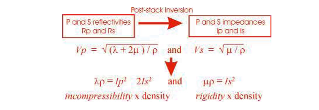
We can go even further to analyze the rocks and fluids within them. With the Fatti P and S impedance attributes (or these same values estimated from other AVO attributes such as Shuey’s NIP and gradient), we can estimate the layer impedances by post-stack impedance inversion (Goodway and others, 1997). This is just the same ‘post-stack inversion’ that we’ve been using for the past couple of decades which turns a seismic trace into a pseudo velocity or impedance well-log. One example of this type of procedure is the so-called ‘sparsespike’ inversion.

Inverting the P and S reflectivities gives us P and S impedances for the geological layers. Taking the common equations for Vp and Vs (which depend on Lame’s parameter, modulus of rigidity and density), we can arrive at simple equations that combine the impedances to arrive at estimates of the elastic properties of the rock. We cannot isolate the density term, but are left with attributes which characterize the incompressibility (LambdaRho™) and the rigidity (MuRho) of the rocks and the fluids in their pore spaces (Figure 10). Note that while the common term for this in the Calgary market is LMR™ the technique is also known as ‘Rock Property Inversion’ (RPI) as well as by other commercial names.

What does this all mean for interpreters? Generally, sandstones are more incompressible than shales. Water filled sandstones are more incompressible than gas filled sandstones. Shales have less rigidity than sandstones. Carbonates can have considerably different incompressibilities and rigidities depending on such things as amount and type of porosity. Changes in fluid would not affect rigidity. Interpretation of these attributes can be very complex (depending on interpretation of well log measured rock physics, cross-plotting and modeling) but they can also be very revealing in those cases (increasingly more common as the easily found reservoirs become rare) where stacked seismic simply cannot differentiate lithologies and fluids.

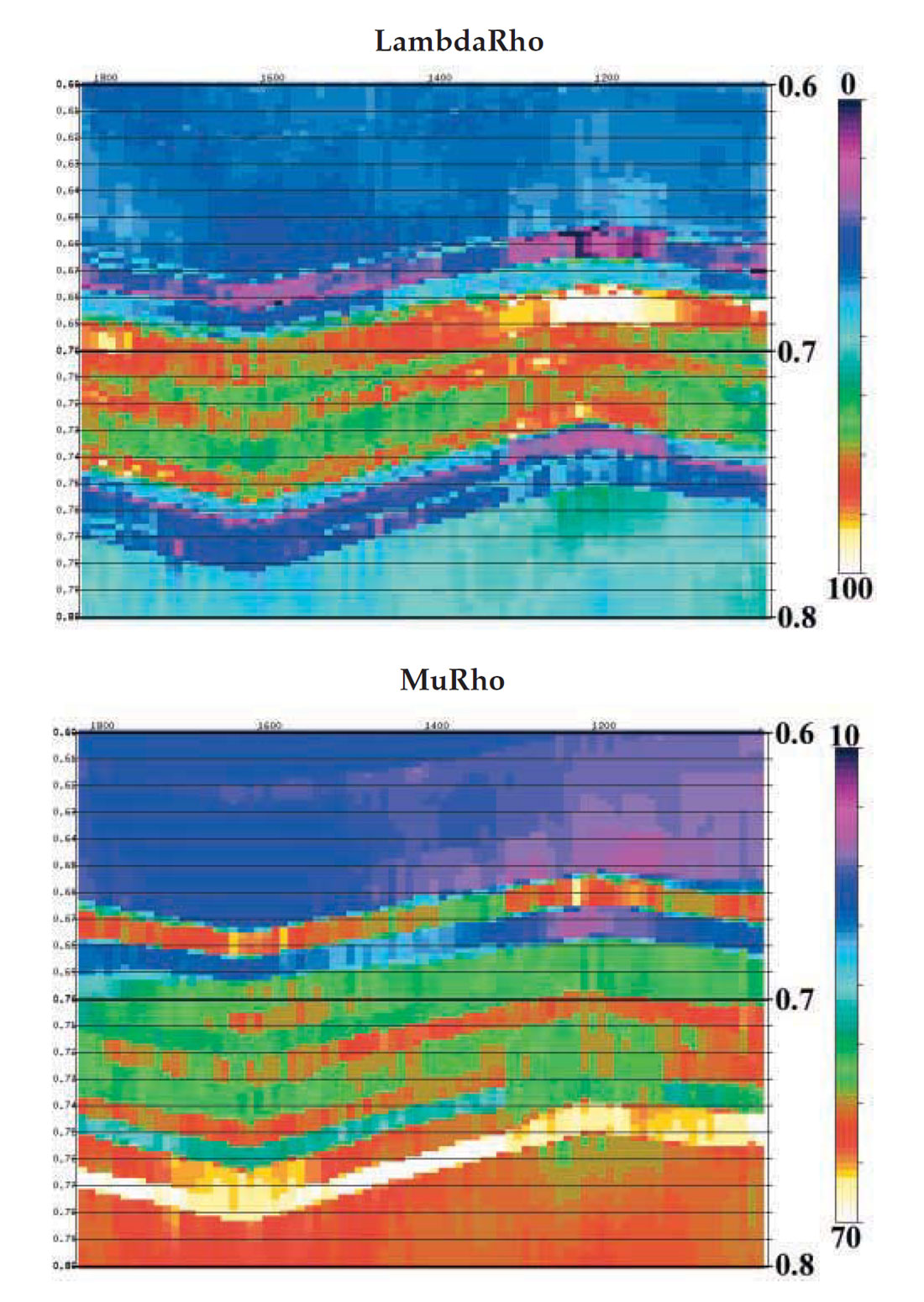
For our model example, we’ve calculated LambdaRho™ and MuRho (Figure 11). As we might expect, the gas sands show relatively lower values of LambdaRho™ and relatively little variation in MuRho. Here, the interpretation is straight forward, but the real world can often be more perversely difficult.

Real Data Example

Now we can look at a real data example from the Cretaceous Bluesky formation from northeastern British Columbia. The first display (Figure 12) is regular seismic stack with four well locations marked. The Bluesky does have well recognized stacked amplitude behavior, but can still be very ambiguous. We’ve extracted the P and S reflectivity sections by use of Fatti’s AVO method, inverted to P and S impedances and then estimated LMR™ layer attributes. In Figure 13 we show the LambdaRho™ section and the Lambda/Mu ratio stack, another attribute that can help to differentiate different fluids and lithologies more easily.

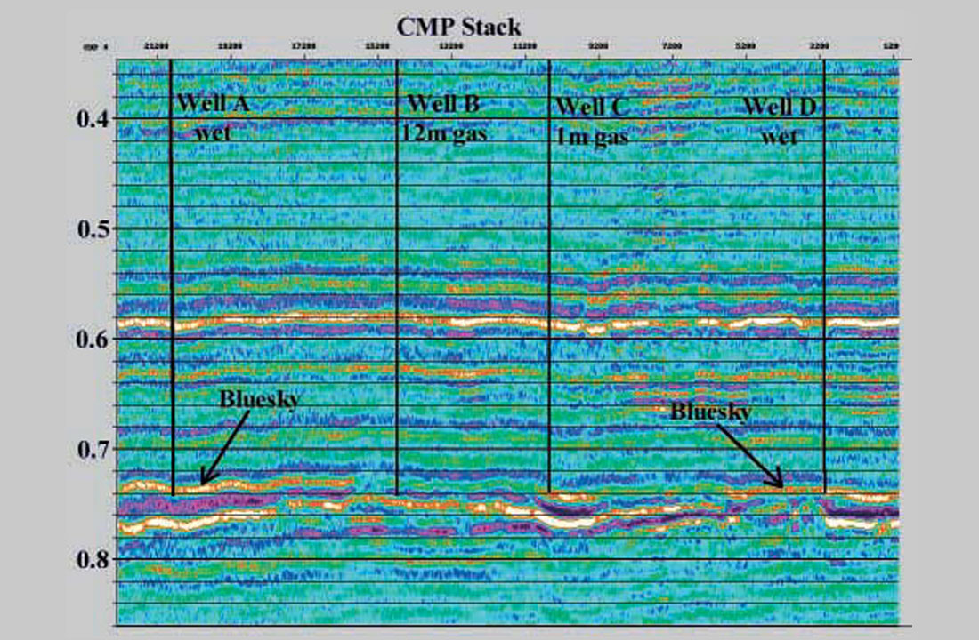
One question often asked about LMR™ analysis is, “What do we do with the results?” In this particular case, we’re looking to distinguish gas sands from water filled regional rocks. We are looking for relative lows in LambdaRho™ with corresponding lows in the ratio display, a usual indicator of gas sands. In this Bluesky example for instance, we see low LambdaRho™ and ratios at the appropriate level at three well locations (Figure 13).

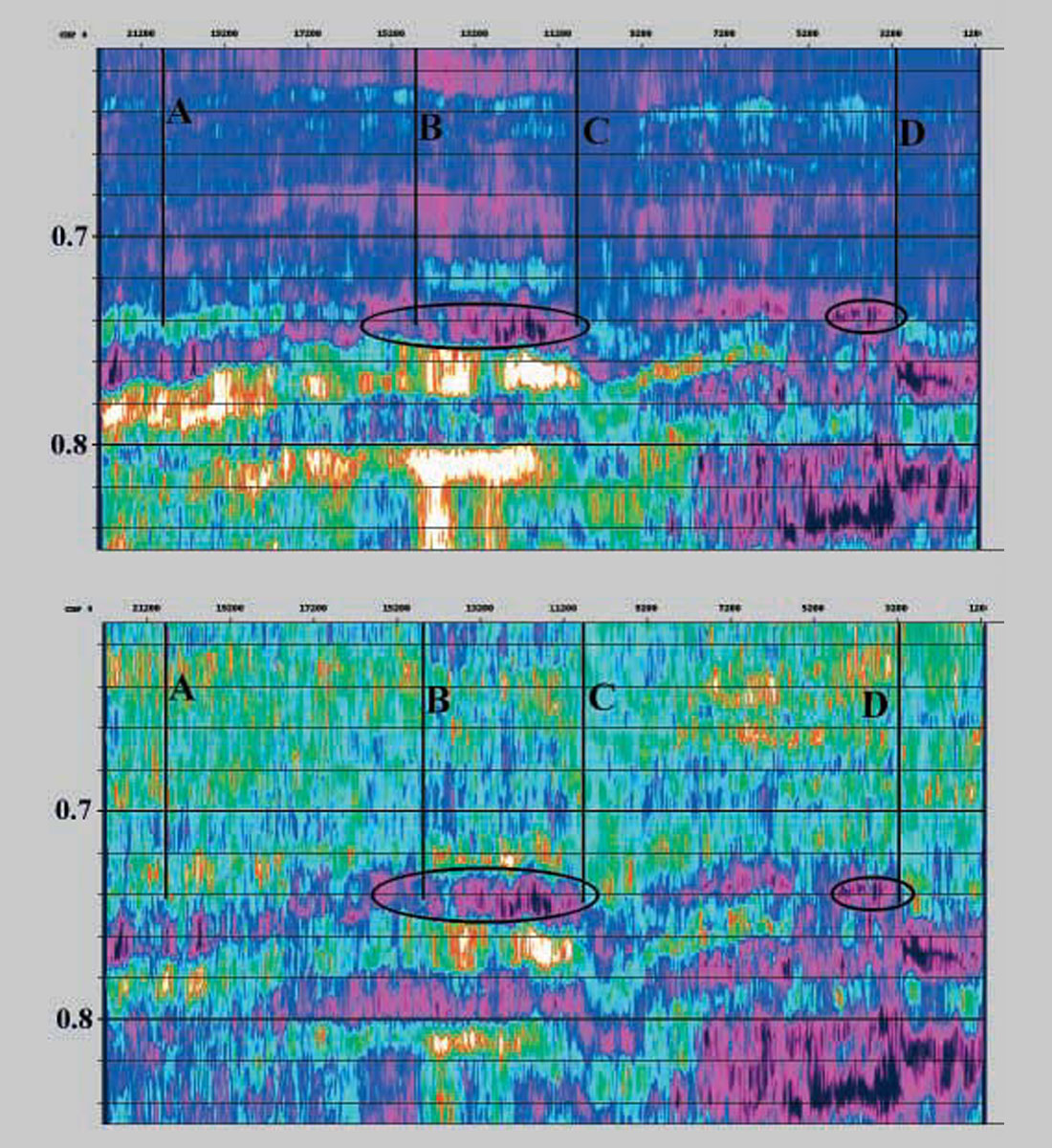
As useful as this approach is, it can be too simplistic. It turns out that one of these locations with prospective rock properties is actually wet. This illustrates the fact that LMR™ interpretation is not always straightforward. Now we have turn to more sophisticated interpretation methods such as cross-plotting. In the final display, we crossplot LambdaRho™ against Lambda/Mu ratio. Despite the similarities in the section displays, the cross-plot shows quite decisively the differences between the gas wells and the wet case.

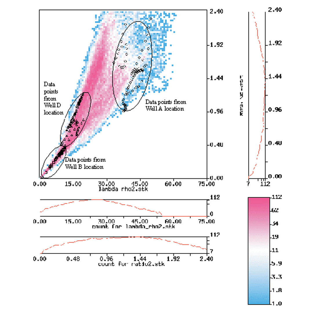
Proper interpretation of seismically derived rock properties consists, in part, of crossplotting different attributes (LambdaRho™, MuRho, ratio, difference, etc.) and analyzing them with a clear understanding (derived through rock physics log analysis and modeling) of what response is expected for the particular geology we are investigating.

Conclusion

Amplitude variations with offset seen on seismic data are due to contrasts in elastic rock properties. These amplitude responses can be easily described by linear AVO attribute extraction and can be used to infer changes in the rocks. Finally, these AVO attributes, combined with post-stack inversion techniques, can give us rock properties which quantitatively characterize the lithology and fluid content of reservoirs.

Acknowledgements

I’d like to thank Jon Downton and Jan Dewar whose work part of this article is based on. Jan Dewer, Kristen Macleod, Florence Janzen and Glen Larsen all made valuable comments on this work.