All roads lead to Rome: predictability, sparsity, rank and pre-stack seismic data reconstruction

In recent years researchers at universities, processing and oil companies have proposed several pre-stack seismic data reconstruction algorithms. In essence, all these algorithms are developed under a common assumption: there is sufficient simplicity in the observed seismic wavefield to permit its representation in terms of a finite number of basis functions. When the representation is in terms of complex exponentials, we have a family of methods that are categorized under the broad field of Fourier reconstruction. The goal of this presentation is to review and connect currently used methods in industry. We would also like to make the claim that all methods invoke simplicity in the wavenumber domain and finally, we will demonstrate that Fourier methods are also connected to methods that are based on prediction error filtering and rank-reduction. In other words, all interpolators operate under the classical assumption that in a small multidimensional patch, data are represented via a superposition of plane waves.

Introduction

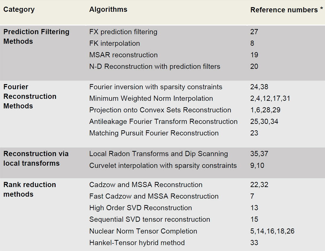
It is difficult to provide a complete survey of reconstruction and interpolation methods in a concise introduction. Running the risk of creating animosity, we included Table 1 where we tried to categorize the main methods for interpolation and seismic data reconstruction. We have also included main references for each category and please, forgive our ignorance if we have missed important references. Clearly, this is not the complete realm of work done in the field, but we believe it captures the main ideas and algorithms that permit the reconstruction of seismic wavefields.

Our claim is that all methods for seismic data reconstruction must assume a high level of parsimony in the wavefield that one desires to reconstruct. In other words, the observations must be represented via a simple regression in terms of known basis functions. The latter is the foundation of methods based on Fourier synthesis where one assumes that the observed seismic data can be represented in terms of a superposition of complex exponentials (Hindriks and Duijndam, 2000). The representation itself is not sufficient to properly honor the data and produce accurate synthesis of unobserved data. This is why the decomposition must be in terms of a limited number of complex exponentials. Methods based on an assumption of sparsity have been successfully adopted to retrieve Fourier coefficients (Sacchi et al.., 1998; Zwartjes and Gisolf, 2007) that permit the proper reconstruction of wavefields within multi-dimensional windows. Minimum weighted norm interpolation (MWNI), applies a less stringent constraint to the data and leads to solutions that are quite similar to those that one can estimate via sparse inversion (Liu and Sacchi, 2004; Trad 2009; Cary 2011, Chiu et al., 2013). However, an advantage of MWNI is that because the concept of sparsity is not invoked, it resorts to a simple algorithm based on quadratic regularization with pre-conditioning. In fact, MWNI should be the optimal regularization technique if one were to know the power spectral density of the data to be reconstructed. However, because the power spectral density is unknown, MWNI uses different strategies to bootstrap it from the data. The latter leads to an algorithm that is extremely similar to sparse inversion solutions via Iteratively Re-Weighted Least-squares (IRLS). Sparse Fourier inversion and MWNI, therefore, can be considered as similar ways to fit data via the superposition of a finite number of complex exponentials. They both can be generalized to multidimensional problems, and clearly, they both have problems with regular grids since they are affected by aliasing. However, patches of seismic prestack data often have enough irregularities to attenuate aliasing making MWNI a robust method for interpolating data on irregular grids (Trad, 2009).

Methods based on algorithms utilized in radio astronomy (the Clean Method of Schwarz, 1978) have also been proposed to regularize seismic data. Examples of the latter are the Antileakage Fourier Transform (ALFT) (Xu, et al., 2005; Schonewille et al., 2009) and Matching Pursuit Fourier reconstruction (MPFR) (Özbek et al., 2009). These techniques find and retrieve one wavenumber at a time to synthesize a spatial plane wave. The latter is removed from the original data and the process is continued until no significant energy is observed in the residual signal.

In essence, the assumption of simplicity (sparsity) is also invoked by ALFT and MPFR methods as they also try to construct a synthesis by the superposition of a limited number of wave-numbers. Both methods have the ability to cope with data at irregular grid positions. When the data are on a regular grid, dip scanning methods can be applied to identify true wavenumbers from their associated alias components (Naghizadeh, 2012). At this point, it is important to mention that both Sparse Fourier inversion methods and MWNI can operate both with regular grids and irregular spatial positions. In the first case, the algorithms can be implement via the FFT engine, whereas in the latter, it is necessary to utilize fast implementations of non-uniform DFTs (Jin, 2010). Finally, we would like to mention POCS, another Fourier method that synthesizes data in terms of, again, a parsimonious distribution of spectral coefficients (Abma and Kabir, 2006; Wang et al., 2010; Stein et al., 2010). POCS uses a Fourier domain amplitude threshold to represent the data also in terms of a simple distribution of spectral amplitudes. In general, POCS, ALFT, MPFR, and MWNI should produce results that are similar because, after, all they are developed under similar assumptions: simplicity (sparsity) of the data representation in terms of spatial plane waves. Most differences between these techniques are probably attributed to implementation and developers ways to cope with geometries, input/output, and data preconditioning. A plethora of tricks is often used to stabilize and bring these algorithms to the realm of industrial applications. For instance aliasing and its solutions for MWNI and POCS have discussed by Cary and Perz (2012) and Gao et al. (2013).

A superposition of complex exponentials (the assumption made by Fourier reconstruction methods) leads to the linear prediction model. In other words, the superposition of complex exponentials immersed in noise can be represented via autoregressive (AR) models. These models are the basis of linear prediction theory, where one states that observations at one channel are a linear combination of observations of adjacent channels. This is also the principle behind FX noise attenuation via prediction filters. The superposition of complex sinusoids in FX (linear events in TX) leads to predictability via AR models in X for a given frequency F. This model is astutely exploited for denoising and for reconstruction (Spitz, 1991; Gulunay 2003; Naghizadeh and Sacchi, 2007). The advantage of FX prediction filter methods is that they can cope with aliasing. In addition, they can be generalized to N-D cases (Naghizadeh and Sacchi, 2010). Again, the assumption is that the data can be represented via a superposition of plane waves that admits representation in terms of an autoregressive model. For this to be true, one needs to segment the data in small spatio-temporal windows to guarantee the validity of the plane wave assumption. This is also a problem we encountered when reconstructing data with Fourier reconstruction methods.

Lastly, we mention rank reduction based methods. In essence, these methods also assume a superposition of linear events. In this case, multidimensional data embedded in a Hankel matrix is used to form a low rank matrix. An algorithm with similarity to POCS is adapted to retrieve a low rank Hankel approximation that fills in missing observations (Trickett et al., 2010, Oropeza and Sacchi, 2011). In the absence of noise or missing data the Hankel matrix of the data is a low rank matrix. In general, the rank is equal to the number of dips in the data. Removal of traces and addition of noise leads to a Hankel matrix that is of high rank. Therefore, the algorithm recovers the missing data by assuming the ideal data to be reconstructed is a low-rank approximation to the ideal fully sampled data. Initial efforts in this area relied on low rank approximations using Hankel matrices and block Hankel matrices. However, recently efforts have shifted to operate directly on multidimensional arrays (multi-linear arrays or tensors) via the concept of low rank tensors. In this regard, one can expand rank-reduction methods for matrices (SVD) to tensors (multi-dimensional arrays) by methodologies like the Higher-Order SVD (Kreimer and Sacchi, 2012a; Silva and Herrmann, 2013), sequential SVD (Kreimer, 2013), or nuclear norm interpolation methods (Kreimer and Sacchi, 2012b, Ma, 2013, Kreimer et al., 2013; Ely et al., 2013). Rank reduction methods that utilize tensors tend to have less stringent constraints on curvature than rank reduction methods based on Hankel matrices. In other words, they can cope with the problem where the waveforms one desires to interpolate have dips that vary in space.

Connection between methods

In general, all reconstruction methods are based on the assumption of simplicity of the representation of the waveform. For instance, a superposition of linear events has a sparse representation in the frequency-wavenumber domain, similarly a superposition of linear events is predictable in the frequency-space domain, and finally a superposition of linear events leads to low rank Hankel structures. In this regard, one can claim the linear event model is behind all reconstruction methods for multidimensional signals. In practice, a linear superposition of events can be safely assumed by windowing the data or by using localized transforms (Hennenfent and Herrmann, 2006; Herrmann and Hennenfent, 2008; Wang et al., 2010)

Examples

To illustrate the similarity of reconstruction algorithms we consider three methods: Projection Onto Convex Sets (POCS), Minimum Weighted Norm Interpolation (MWNI), and a rank reduction method for tensors called Sequential Singular Value Decomposition (SEQSVD). Both MWlNI and POCS are transform-based methods that operate in the multidimensional F-K domain. POCS searches for a solution via convex optimization by iteratively thresholding the amplitude spectrum of the data (promoting sparsity) and resetting traces at original trace locations to their input value (Abma and Kabir, 2006). MWNI searches for a solution using linear inverse theory. A solution is sought that minimizes a weighted norm in the FK domain (promoting sparsity), while minimizing the misfit between observed data and the data synthesized using the FK domain model (Liu and Sacchi, 2004). SEQSVD is a rank based technique that operates in the multidimensional F-X domain. For 3D data rank-reduction is applied to each frequency slice of the data and traces at original locations are reset to their input value (identical to the POCS imputation algorithm). The rank reduction is carried out via the Singular Value Decomposition (SVD). The SVD factorizes an mxn matrix D into three matrices: UΣV^T.

The m columns of U are called the left singular vectors, the n columns of V are called the right singular vectors, and the values lying along the diagonal of the mxn matrix Σ are known as the singular values of D. Rank reduction is achieved by zeroing low amplitude singular values and performing matrix multiplication of UΣV^T. For higher dimensional data each frequency slice must first be unfolded into a matrix before rank reduction and re-folding to original dimensions. An example of this unfolding is shown in Figure 1, where a three dimensional tensor is unfolded into a two dimensional matrix. This unfolding should be repeated for all possible unfolding configurations (Kreimer, 2013).

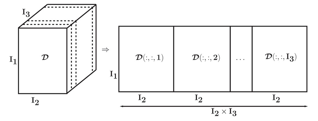
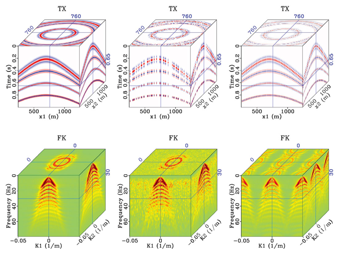
Figure 2 shows a synthetic 3D common shot gather and its associated FK spectrum. The data have been decimated in two different ways. In the middle column, 50% of the traces have been randomly decimated, leading to an FK spectrum that has scattered, low amplitude noise. Imposing sparsity on this spectrum (as is done in POCS and MWNI) leads to solutions that can fill in the missing traces. In the right column every second trace in both spatial dimensions have been regularly decimated, leading to and FK spectrum that has regular aliases with the same amplitude as the signal we wish to reconstruct. Imposing sparsity alone will fail to fill in the missing traces; additional constraints for anti-aliasing are needed to reconstruct the missing traces.

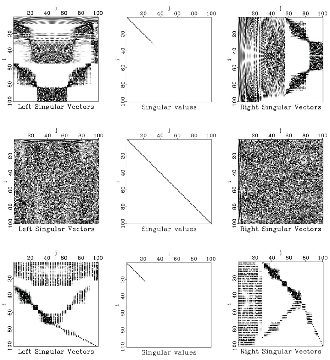
To make an analogy between the use of the FK transform (used by POCS and MWNI) and singular value decomposition (used by SEQSVD), Figure 3 shows the singular value decomposition of the data from Figure 2. Each frequency slice from the true data is decomposed into a matrix of left singular vectors (left column), a matrix containing singular values along the diagonal (middle column), and a matrix containing right singular vectors (right column). When the data are randomly decimated (middle row), the highest-amplitude singular values are spread along the diagonal of the matrix. Imposing low rank (keeping only the highest amplitude singular values) we can fill in the missing traces in the data. When data are regularly decimated we have completely missing fibers (missing “columns” or “rows” in a higher dimensional sense) contributing to the matrices of left and right singular vectors, and the rank remains the same as the original data. Imposing low rank in this case will fail to reconstruct the missing traces.

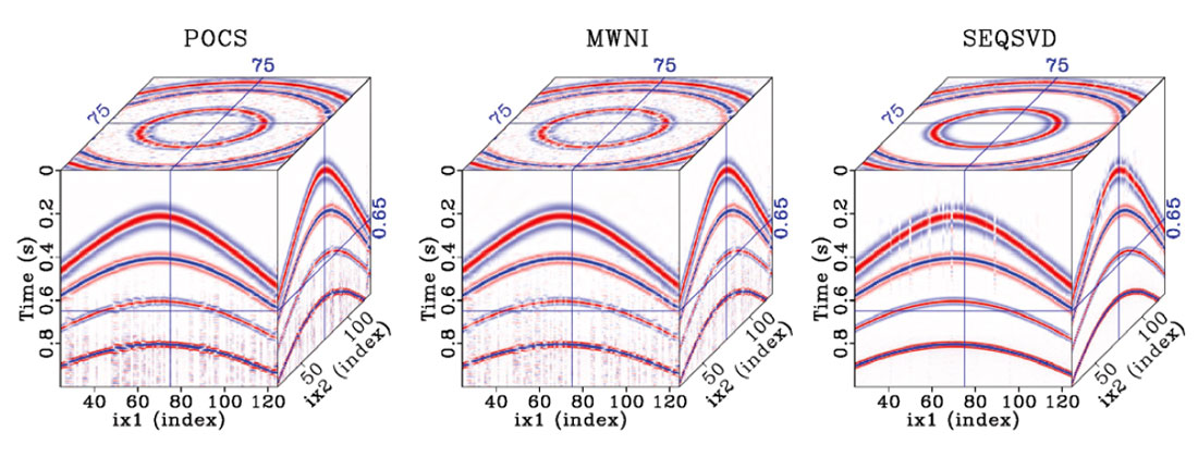
Despite the difference between these algorithms, they can provide similar reconstruction results. Figure 4 shows the application of POCS (left), MWNI (middle), and SEQSVD (right), to the randomly decimated data shown in Figure 2. All three methods provide similar results, although SEQSVD slightly outperforms POCS and MWNI due to its unique ability to handle curved events. While Fourier reconstruction methods represent curved events via a superposition of plane waves, rank based methods that utilize tensors assume a linear combination of complex exponentials. This is a more general representation than plane waves: each event could have a different relation with respect to each axis (dimension), which allows for low rank representations of both linear and parabolic events as well as events of any other function that admits separability in the FX domain. Although seismic data are typically NMO corrected prior to reconstruction, the ability of SEQSVD to better reconstruct curved events could offer an advantage in the reconstruction of diffractions, or even in reconstructing data that can not be NMO corrected, such as data from simultaneous source acquisition.

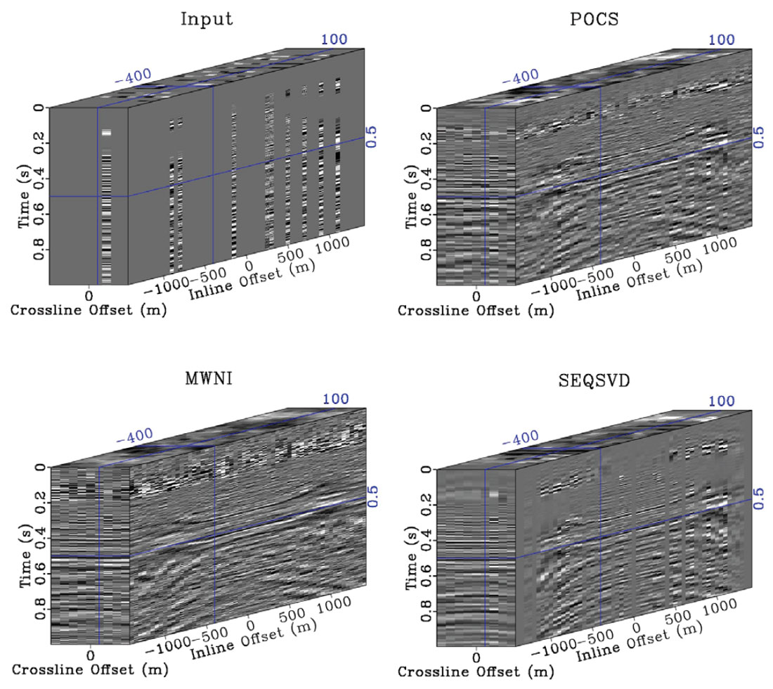
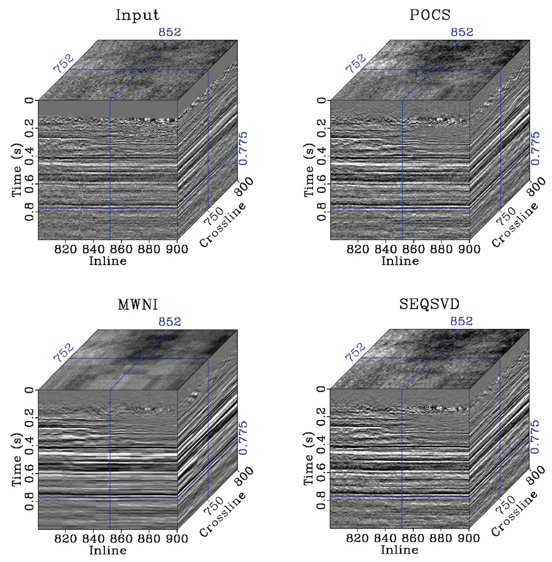
Our final example is from a land dataset in the WCSB. It is a heavy oil play with little structure, although the input data are sparse and noisy. The data are binned on a 10x5m CMP grid, and a 100x50m Offset-X-Y grid prior to interpolation. The data are broken into patches of 10x10 CMPs and 200 time samples for computation memory/time and stationarity. An average patch of data contains 85% missing traces. Figure 5 shows a single CMP bin for input data, POCS, MWNI, and SEQSVD 5D reconstructions. The results from the three methods appear quite similar, although the result of SEQSVD contains several low amplitude traces associated with completely missing fibers in the original 4D spatial tensor structure. It should be noted that all three methods in these cases are “vanilla” implementations of the algorithms. By weighting the F-K spectra (in the case of POCS and MWNI), or otherwise dealiasing the rank reduction operation in SEQSVD (an active research topic) these results could be made even more similar. Figure 6 shows the stacked results for each reconstruction method. Again, the results are very similar for each of the methods, although MWNI is slightly smoother than the other two methods. Similar results could be achieved by re-parameterizing the preconditioning in MWNI to have less sparsity promotion, or by decreasing the weighting of the original data during the imputation step of the POCS and SEQSVD algorithms.

Conclusions

At the heart of all reconstruction methods lies Occam’s razor: the assumption that the simplest model should be chosen over more complicated ones. This is a powerful assumption that is used in many fields outside of Geophysics (even Science). For example, in Geology the principle of lateral continuity assumes that sedimentary layers can be assumed to extend laterally in all directions. This assumption becomes useful when mapping lithology in the presence of erosional features. In reconstruction the assumption of simplicity can take different forms: in prediction filtering methods we assume the data can be modeled in an autoregressive fashion, while Fourier synthesis methods assume sparsity in the FK domain. Finally, rank based methods assume that noise and missing traces increase the rank of the data, and by reducing the rank we can recover the underlying signal.