Over the last decade, Airborne Electromagnetics (AEM) has become a widespread tool for groundwater applications. Besides the demand of acquiring good quality AEM data, there are two other fundamental steps to obtain a robust geological and hydrogeological model: accurate processing/inversions and advanced interpretation.
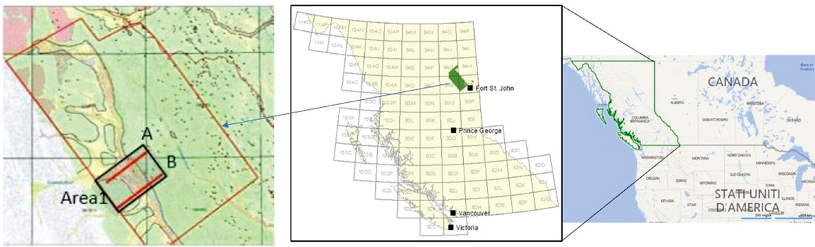
We show the results achieved adopting this approach, on a subset of a large AEM survey within the Peace Project, in British Columbia, Canada (www.geosciencebc.com/s/PeaceProject.asp). This project is a collaborative effort involving Geoscience BC, the Ministry of Forests, Lands and Natural Resource Operations, the Ministry of Environment, the BC Oil and Gas Commission, the Ministry of Natural Gas Development, BC Oil and Gas Research and Innovation Society (BC OGRIS), Progress Energy Canada Ltd. (now Petronas Canada), and ConocoPhillips Canada, with additional support from the Peace River Regional District and the Canadian Association of Petroleum Producers.
This paper (largely based on Viezzoli et al., 2018) is the natural continuation of the Best et al. (2017) December 17 RECORDER issue, in which they presented the results of the integration between AEM inversion results and gamma logs.
AEM data were acquired by SkyTEM Aps on behalf of Geoscience BC. Approximately half of the survey was later processed and inverted by Aarhus Geophysics Aps. Finally, GEUS (the Geological Survey of Denmark and Greenland) carried out a hydrogeological interpretation on a yet smaller subset. The whole prospect covers approximately 21,000 line km and we present the hydrogeological modeling for a subset of the survey area, located in the north-west (Figure 1) that corresponds to about 2000 km2 (i.e. approximately 4500 line km).
From a hydrogeological point of view, the main target is the detection of buried valleys, since they hold the most promising potential for sustainable groundwater production in the area.
Geological setting
Restricting our attention to the geological formations present within the expected penetration depths of the SkyTEM method (approximately 2 to 400 m in this geology), we identify, from older to younger: the Nordegg Formation (calcareous mudstones), the Buckinghorse Formation (shales, silty mudstones and siltstones), the Sikanni Formation (sandstones and siltstones), the Sully Formation (shales and siltstones) and the Dunvegan Formation (sandstone with subordinate conglomerates). The potential bedrock aquifers are represented by the sandstone units within the Sikanni and Dunvegan, together with the conglomerate lenses within the latter.
The Quaternary sequence is composed of glacio-fluvial deposits (sands, pebbles and gravels), glacio-lacustrine deposits (silty clays or clayey silts), tills, colluvial (sandy and clayey silts) and fluvial units (mainly sands and gravels). The sequence is generally quite thin outside the paleovalleys. The paleovalleys show thick sequences of often coarse-grained infill sediments that might constitute promising aquifers. However, we must pay great attention to the relationships between these shallower aquifers and any potential contaminant coming from the surface, as they are more vulnerable from an environmental point of view. At the same time, many of the paleovalleys are situated directly beneath the modern riverbed. Groundwater extraction from these areas might therefore influence the rivers markedly. Hence, correct hydrogeological modeling is mandatory to responsibly manage the groundwater resources.
The table below reports the expected resistivity ranges (from downhole resistivity logs) of some of the main formations encountered in the area.
| Formation | Resistivity |
|---|---|
| Glaciofluvial deposits | ~ 100 Ωm |
| Glaciolacustrine deposits | ~ 10 Ωm |
| Dunvegan Formation | ~ 50 Ωm |
| Sully Formation | ~ 15 Ωm |
| Sikanni Formation | ~ 30 Ωm |
Methodology
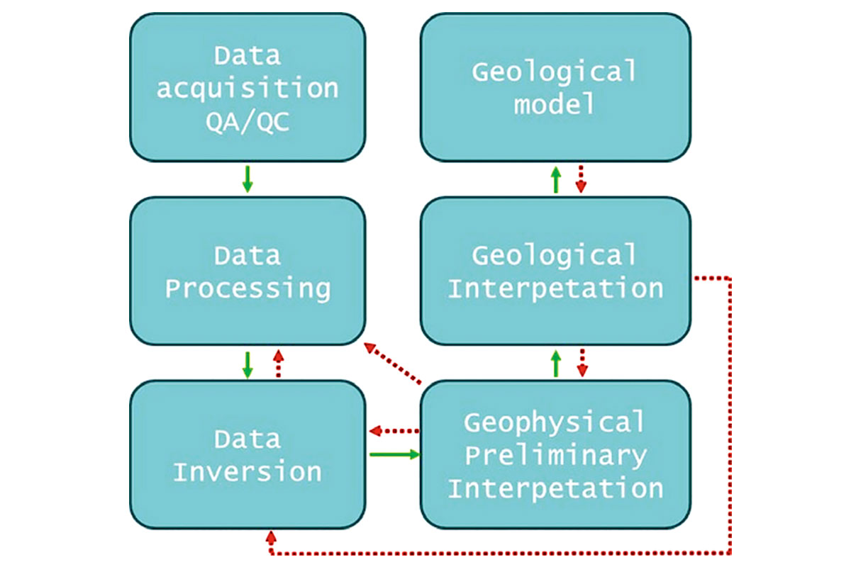
Figure 2 shows the schematic of the overall workflow adopted in this project. Notice how it is not unidirectional, but iterative, with preliminary results from later steps feeding back into previous steps, for fine tuning. Especially important is the close cooperation between geophysicists and geologists. The goal is to obtain a geological model consistent, at once, with all sources of information (and their respective uncertainties): geophysical data, geophysical models, prior geological information (e.g., drilling), and conceptual geological model.
Data acquisition, processing and inversions
SkyTEM is a time-domain helicopter electromagnetic system designed for hydrogeophysical, environmental and mineral investigations. The SkyTEM system is composed of a transmitter (12 turns, 337 m2 eight-sided loop) and a z-component receiver (placed approximately 2 m above the frame). The system makes use of both a Low dipole Moment (LM) and High dipole Moment (HM) that yield both near surface and deep resolution.
Data are subject to QA/QC procedures at the end of each flight. This survey (21000-line km) was finalized in approximately 6 weeks, with 2 SkyTEM systems. After acquisition, the data is processed. The processing largely follows Auken at el. (2009).
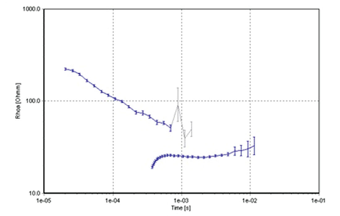
Soundings were averaged over 1.4 s of flying, corresponding to approximately 30 m separation between soundings. The resulting data density greatly helps the geological-hydrogeological interpretation. Figure 3 shows an example of a TEM sounding, shown as apparent resistivity vs time, with different time gates displaying different noise levels for the low and high moment.
The AEM and navigation data are first processed to eliminate cultural artefacts and improve signal to noise ratio. The fundamental task, carried out utilizing a combination of automated and manual procedures, prevents artefacts in the resistivity and hydrogeological models, as shown by Viezzoli et al. (2013).
Final inversions are carried out using the quasi 3-D Spatially Constrained Inversion (SCI) (Viezzoli et al., 2008). Using constraints across model parameters, which are tied together with a spatially dependent covariance, the SCI returns the spatial variability expected in the local geological setting. The flight altitude is included as an inversion parameter with a prior value calculated from the tilt corrected laser altitudes. The Depth of Investigation (DOI, Christiansen and Auken, 2012, based on the sensitivity to the model parameters, was calculated as the last step of the inversion. It is a crucial ancillary QC and is most useful when inspecting and interpreting results at depth.
Geophysical Results
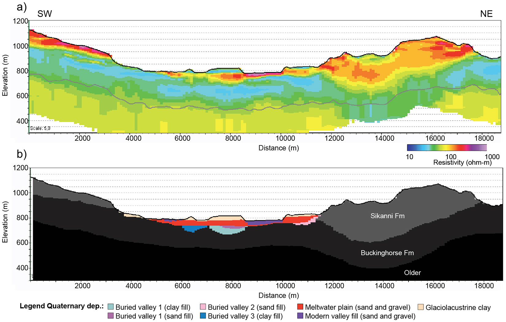
The inversion results are compared with the existing boreholes. The resistivity cross-sections of Figure 4 show a couple of examples, with the stratigraphic data represented essentially by the thickness of Quaternary sediments and depth to and type of bedrock.
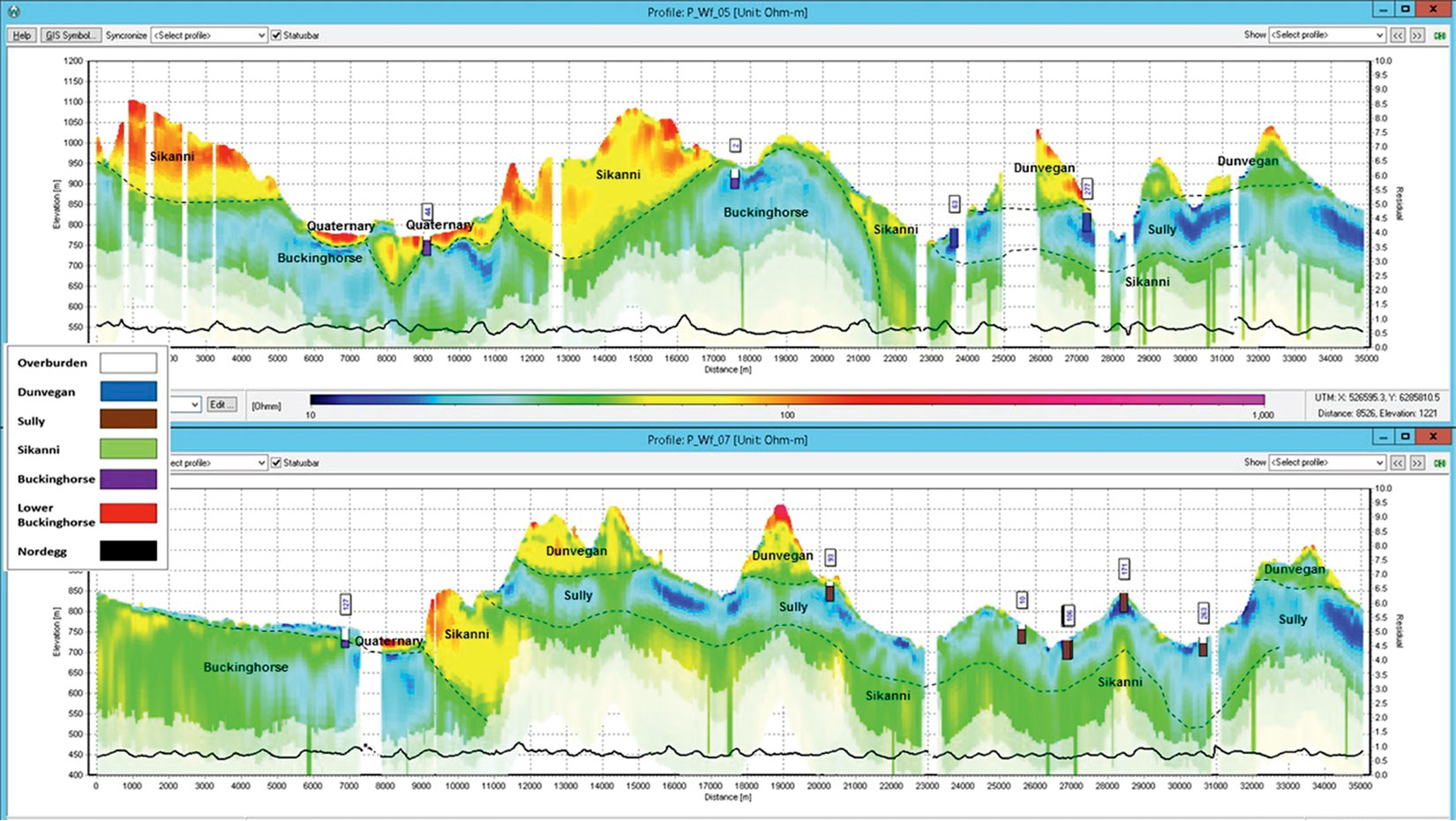
Even though the resistivity values for the different lithological formations estimated from the logs only show small differences (Table 1), the lithological formations seem to be easily distinguished in the SkyTEM’s derived resistivities. Thus, the Sully and Buckinghorse formations show low resistivities due to the presence of shale, whereas Sikanni and Dunvegan show high resistivities. The capability to distinguish different bedrock formations allowed delineating a complex structural framework (Figure 4).
Depth to bedrock is generally well resolved both shallow and deep. See for example the good agreement between the boreholes around 9000 m for the top cross-section and at 7000 m for the bottom one. The Quaternary units can display a sharp conductive feature where glaciolacustrine deposits prevail, or a rather resistive response, linked to buried valleys filled with gravels and sands.
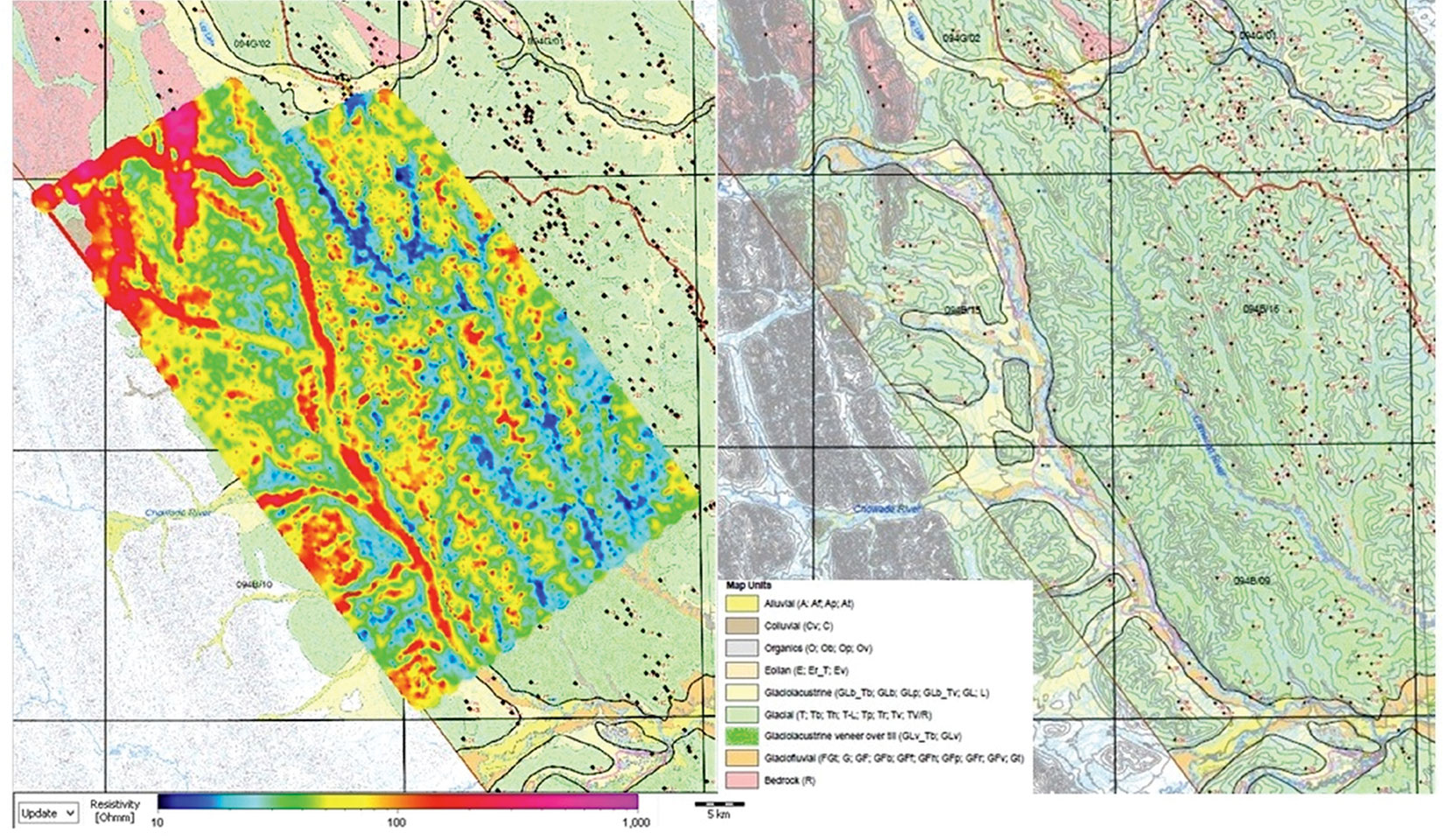
Figure 5 displays the correlation between outcropping geology and shallow resistivity (0-5 m depth), confirming the electrical response of the geological formation: note the elongated resistive deposits associated with the fluvio-glacial or the alluvial deposits within the Halfway River and its tributary Chowade River. On the contrary, the finer glacial till is characterized by lower resistivity. In the northwest corner of the map it is possible to recognize the typical resistive response of the Nordegg Formation that is the only bedrock unit outcropping in this area and that is marked as “bedrock” in this geological map.
Geological interpretation
Interpretation of the AEM data reveals a highly complex structural setting, where the bedrock formations show large-scale folds and thrust structures (Figure 4). Additional structural information can be derived from the results (see Jørgensen et al., 2017, 2018), but this paper will mainly focus on the mapping and modelling of paleovalleys, due to their groundwater extraction potential.
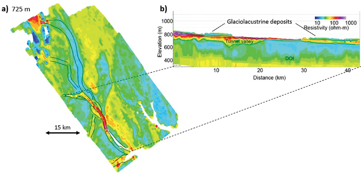
A number of paleovalleys have been mapped in the study area (Figure 6a). The paleovalleys are recognized in the AEM data as elongate resistivity structures that broaden upwards. Most of the paleovalleys are situated along the modern valleys stretches, but others are detected in hilly areas. The buried valleys occur in at least two generations. The first generation has overdeepened sections along their thalwegs and may therefore be interpreted as subglacially formed tunnel valleys that later have been infilled with younger sediments. This type of buried paleovalleys are frequently found within all formerly glaciated areas (Jørgensen and Sandersen, 2006; Kehew et al., 2012). The formation of the second generation of buried valleys is connected to the recent fluvial erosion and deposition of pebbles and gravels in the riverbed. The second generation of valleys are limited in depth and are found beneath many stretches of modern rivers, such as the Halfway River and its tributaries (Figure 5).
A profile along the southern paleovalley is shown in Figure 6b. The valley shows an undulating bottom profile that is characteristic of subglacially formed valleys. The valley is up to 100 m deep at its deepest depressions and shows high-medium resistivities at depth. In the northern part of the valley (profile distance 0 – 20 km), very high resistivities are seen in the upper part. Here, the older valley has been cut by the younger, fluvial erosion and deposition of coarse-grained gravels and pebbles. Low resistivity deposits are recognized on top of the paleovalley structure in many places. These low resistivity deposits are glaciolacustrine clay that covers large parts of the modern river valley (Figure 5b, Petrel Robertson, 2015).
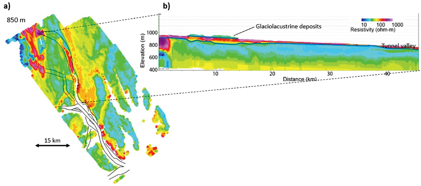
The second long paleovalley is found beneath the northernmost stretches of the Halfway River Valley (Figure 7). It can be followed until it crosses Pink Mountain in the north. This valley is up to about 75 m deep in its northern part (Figure 7b, profile distance c. 10 – 15 km). These valleys have subsequently been cut by modern river streams along large sections of their length and in these sections it is difficult to distinguish between the modern river sediments and the older paleovalley fill. The uncertainty of the interpretations is thus relatively high here.
Geological modelling
A geological model was constructed for a subset of the area. The model is constructed based on a cognitive approach, in which all available data (surface geological map, stratigraphic boreholes, AEM data, terrain, etc.) and the overall conceptual geological knowledge are combined and translated into a manually interpreted 3D voxel model (see also Høyer et al., 2015; Jørgensen et al., 2013).
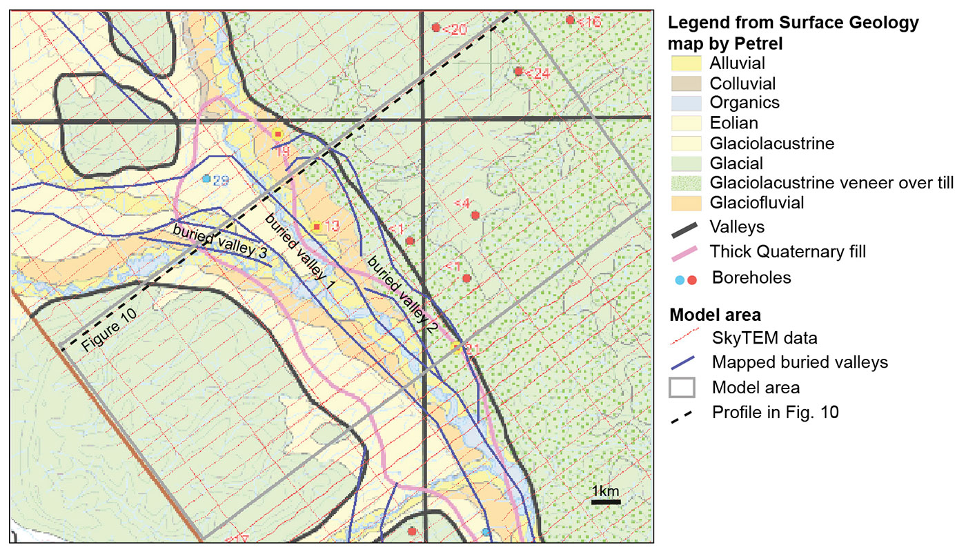
The 3D geological model was constructed using the geological software modelling tool ‘Geoscene3D’ from I-GIS (2018). The model area (Area 1 in Figure 1) covers a section of the long paleovalley that follows the southern part of the Halfway River Valley (profile distance 10 km to 18 km in Figure 6b). In the following, this valley is named ‘Buried Valley 1’. Figure 8 shows a close-up of the surface geology map in the model area together with the outline of the interpreted buried valleys and the position of the profiles in Figures 10.
The geological modelling is performed using a combination of layer- and voxel modelling tools using a similar approach as the geological modelling of buried valleys in Høyer et al. (2015) and of Sapia et al. (2015). The bottom of each geological unit is modelled using interpretation points that have been kriged into surface layers. The bottom of four overall stratigraphic boundaries have been modelled; Buckinghorse, Sikanni, Sully and Dunvegan Formations. In the valley, the bottom of six Quaternary boundaries have been modelled; Buried Valley 1, Buried Valley 2, Buried Valley 3, the Meltwater Plain, the Modern Valley Fill and the Glaciolacustrine Deposits.
Subsequently, a voxel model is constructed by using the tools described in Jørgensen et al. (2013). The final voxel model is discretized with 100 m x 100 m laterally and 5 m vertically and covers the elevation interval from 300 m a.s.l. to the terrain surface (up to 1210 m a.s.l.), resulting in about 7.7 million voxels. The voxel model is constructed by selecting and populating voxels within volumes delineated by the modelled layer surfaces and defined regions. Overall, the units correspond to the ones defined by the layer surfaces, but two of the units (‘Buried Valley 1’ and the ‘Dunvegan Fm’) are further subdivided into lithological facies based on the resistivity values within the units (with 60 ohm-m as a cut-off value). The stratigraphic formations are known to be heterogeneous, but due to the greater burial depth of these formations, the SkyTEM data are not able to resolve the small lithological variations, and resistivity values are therefore not used for lithological characterization within these units.
The resulting voxel model consists of 13 categories, which are shown together with the 3D view of the modelling results in Figure 9. The Quaternary deposits have only been modelled within the modern valley structure (Figure 9), since the remaining part of the area generally shows a thin cover of Quaternary sediments (Figure 8), with thicknesses below the vertical discretization in the voxel grid (<5 m). In the modern valley structure, the Quaternary deposits have thicknesses between 20 m to approximately 200 m, where the buried valleys are deepest.
Figure 10 shows the resistivity data together with the model results along the northernmost flightlines within the study area (Figure 8). In the northern part of the model area (Figure 10a) a synclinal structure is recognized east of the valley, whereas a thrust fault structure is recognized below the Buckinghorse Formation in the southern part (Figure 10b). The Sully and Dunvegan Formations are only present in the southeastern part of the model.
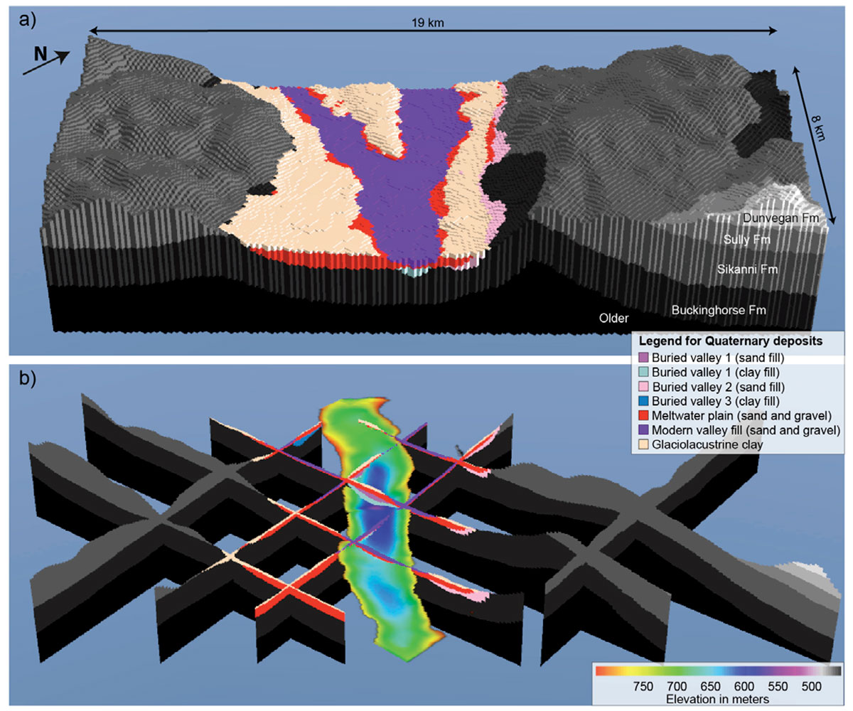
Three buried valleys are modelled within the model area. The largest is the one named ‘Buried Valley 1’. This corresponds to the southernmost long tunnel valley (Figure 5) that is located directly below the modern river in the southern part of the model (Figure 9a,b). In the north, it is located below an erosional remnant of glaciolacustrine deposits (Figure 10, profile distance 7700 m). The lower part of the valley is mainly filled with clayey deposits, whereas the upper part has coarse-grained infill. Close to the hill-side in the eastern side of the modern valley, Buried Valley 2 is located and filled with mainly coarse-grained deposits. Buried Valley 3 is located in the northwestern part of the model area (Figure 10) and is filled with clayey deposits.
All three buried valleys are interpreted to be first generation tunnel valleys that are older than the meltwater plain. The coarse-grained deposits from this unit therefore cut through the buried valley structures (Figures 9 and 10). Glaciolacustrine clays are modelled on top of the Meltwater Plain, and in the north, a marked erosional remnant of these glaciolacustrine deposits forms a small hill structure in the middle of the modern valley (Figure 9a). The youngest deposits in the geological model are the sand and gravel deposits from the modern riverbed, which is cut into the underlying deposits (e.g. Figure 10, profile distance 8500-10,000 m).
Conclusions
A coherent hydrogeological model of a subset of the Peace River SkyTEM survey was obtained through advanced processing, modelling and geological interpretation of the AEM data. Resistivity models provided a new, detailed insight into the local geology, improving the structural and lithological framework. Moreover, thanks to the sharp resistivity contrast, it was possible to map buried valleys, filled with permeable units that could represent important local aquifers.
The highest resistivities are found within the modern riverbed (>100 ohm-m), thus indicating coarse-grained sediments without much clay. The most interesting sites for groundwater extraction could therefore be within the sand-filled parts of the buried valley structures, or in the meltwater plain, where those units are not in direct hydraulic contact with the modern riverbed.
Future work
As Morgan et al. (2017) summarized in their final report, recommendations for future work may include: extending the geological model to the whole area; improving the understanding of the groundwater resource potential of bedrock aquifers; additional geophysical surveys (e.g. seismic, ground-based EM, a SkyTEM survey flown south of the Peace River); additional drilling, including pumping tests, to further geological understanding.

Acknowledgements
The authors acknowledge the in-kind and funding support that the partners of the Peace Project have made to this study.


Join the Conversation
Interested in starting, or contributing to a conversation about an article or issue of the RECORDER? Join our CSEG LinkedIn Group.
Share This Article