Achieving Consistent and Stable Phase with Mixed-Source Surveys

Introduction

So as to minimize the cost of data acquisition, the use of different seismic sources is common in land and marine transition zone surveys. Mixed sources within a survey, however, introduce complications to the data processing effort. Similar difficulties arise when merging 3-D surveys. A key issue to address, in these cases, is shaping reflection events so that the final dataset may be interpreted easily and unambiguously. To achieve this goal, the wavelets representing reflecting interfaces must be broadband, have a known phase, and must be horizontally and vertically stable. The manipulation of seismic data to achieve these desired wavelet characteristics is generally called wavelet processing.

Typically, due to the presence of spatially varying random noise, one uses some form of surface-consistent deconvolution to perform a more stable shaping of the wavelet. For this reason, surface-consistent deconvolution (SCD) is considered a cornerstone of wavelet processing. However, SCD is still subject to the same assumptions made when performing predictive deconvolution, which include that there is a minimum-phase wavelet and there is no noise in the seismic data.

To help quantify the errors introduced by SCD one may employ a methodology called Model-based Wavelet Processing (MBWP).

This approach uses statistical and data-derived information to create a convolutional model of the seismic wavelet. The model accounts for the deleterious effects on predictive deconvolution caused by

• Non-minimum-phase components in the seismic wavelet
• Random noise
• Finite-length predictive deconvolution operators designed with white noise
• Non-white reflectivity

Surface-Consistent Deconvolution

In practice, SCD employs a straightforward methodology to minimize the impact of varying levels of random noise on the deconvolution process. First, the seismic wavelet, w(t), is modeled as a series of convolutions

w(t) = Source * Detector * Midpoint * Offset

Although other terms may be included such as azimuth, the form above is used here. To decompose each term, first transform this equation to the frequency domain so that the convolution is replaced by complex multiplication. Then, by taking the logarithm of the trace power spectra, the surface-consistent model simplifies to

log(W(f)) = log(Source) + log(Detector) + log(Midpoint) + log(Offset).

Conventional surface-consistent decomposition then yields statistical estimates for the different terms. Although random noise is not part of the model, the constraints on the predictive deconvolution operator, imposed by surface consistency, should minimize the effect of noise on the individual terms.

The simple form of the wavelet model highlights several critical issues in deconvolution. First, components of the model might not be minimum phase, a feature that is not properly addressed in classical deconvolution. These non-minimum-phase components are common in mixed-source surveys. Additionally, additive random noise is missing from the model. In a mixed-source survey, the different sources typically exhibit different noise characteristics that further compound the problem. The result is an inconsistent phase result between the different source types after deconvolution.

Model-Based Wavelet Processing

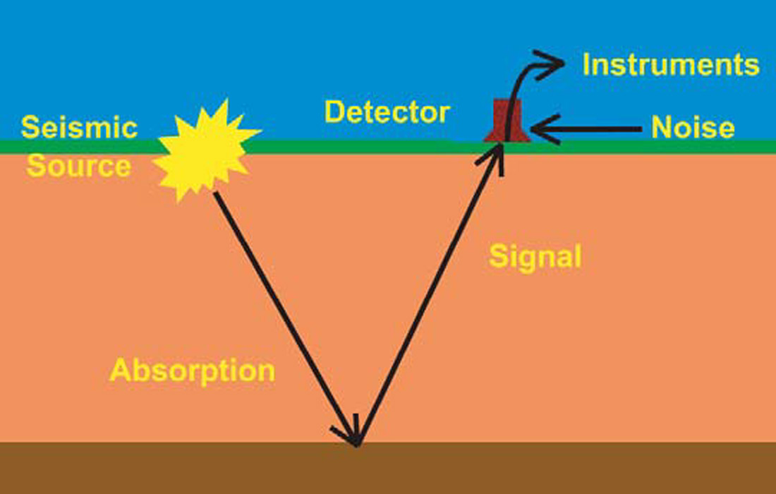
To address the impact of non-minimum-phase components in the seismic wavelet and the effect of random noise on deconvolution, MBWP uses a more sophisticated model for the seismic trace. Consider the schematic of the seismic experiment shown in Figure 1. It depicts a seismic source for the wavelet. This wavelet undergoes attenuation and absorption as it propagates to the reflecting interface and back to the detector. The detector simultaneously receives this signal event and other noise, both of which are recorded by the instrumentation. This suggests the following convolutional model for the seismic data trace

x(t) = ((Source * Q * Reflectivity) + Noise) * Detector * Instrument

Now, random noise is incorporated into the model and absorption is explicitly included as anelastic Q with its frequency- decay of amplitude and, importantly, its minimum-phase filtering action. Note that the model may be written in another form by carrying out the convolutions

x(t) = (Source * Q * Detector * Instrument * Reflectivity) + (Detector * Instrument * Noise).

or in the more compact form

x(t) = σsWs(t)*Reflectivity + σnWn(t)*Noise

Here σs and σn are the signal and noise strengths, respectively. Ws(t) is that portion of the wavelet convolved with the reflectivity and represents the seismic wavelet. Wn(t) contains the noise and represents a source of error in the deconvolution process. In the new model, the terms for source, detector, and instrument may be accurately modeled or are recorded in the field. They represent deterministic components of the wavelet and consequently the model contains any of their non-minimum-phase characteristics. Using the autocorrelation of this model one can examine the effect of noise on the deconvolution operator. It is even possible to examine the influence of non-white reflectivity and noise on deconvolution using this model.

The unknown quantities in the model are the amount of absorption (a value for Q) and the signal-to-noise ratio. These factors are determined via an analysis of the trace spectra that consists of a best-fit match between trace spectra and models for a range of Q values and signal-to-noise ratios. The Q estimate includes the influence of short-period multiples and is therefore an “effective” Q. From the “effective” Q and signal-to-noise ratio analysis, average values of each are used to represent the data.

With all the wavelet variables defined, one can form a model wavelet. The deconvolution parameters used in production processing along with the autocorrelation of the model allow one to compute a deconvolution operator to apply to this wavelet. The operator is then applied only to the signal part of the wavelet estimate. The result is a distorted wavelet that accounts for any non-minimum-phase components in the model and the effect of noise on the design of the deconvolution operator. This wavelet is used to design a residual filter that shapes the distorted wavelet to zero phase. This residual filter (phase only) is then applied to the data after deconvolution.

Merging the data, from a mixed-source survey, takes place after the design and application of MBWP residual filters for each source type. One of the first quality-control tests is a crosscorrelation between stacks of the separately processed source data in the zone of overlap. It is important to realize that no shaping filters have been used to force a fit between, for example, Vibroseis and dynamite data. Each data volume has been independently driven towards zero phase. Typically, the results of the crosscorrelation are a small phase rotation between the two surveys. This is an excellent confirmation of the accuracy of the model-based wavelet processing methodology. Had a forced shaping-filter been used, no such quality control would be possible. If found to be significant, a separate phase correction may be applied to the data prior to final processing.

There are several significant features of Model-based Wavelet Processing. First, the crosscorrelations described above yield essentially independent confirmation of the reliability of the process. Second, the different source types, or different surveys, are independently driven towards zero phase. Consequently, data sets processed independently may be more successfully merged after stack if multiple data volumes are available in a prospect area. This may remove the time needed to reprocess data to achieve a consistent result. Finally, random noise and non-minimum-phase features have been directly addressed in terms of their residual effect on the surface-consistent deconvolution process.

Verifying the reliability of the MBWP estimate of the seismic wavelet can be difficult, since direct observation of the seismic wavelet in surface seismic data is problematical. A Vertical- Seismic Profile (VSP) experiment provides one means for observation of the seismic wavelet. Assuming that reflectivity values are small, the downgoing first-arrival event in the recorded VSP data is an estimate of the seismic wavelet that is propagating in the earth. Similarity of the VSP first arrival and the MBWP model of the seismic wavelet indicate the reliability of the MBWP model.

Figure 2 is a comparison of the MBWP model (the solid lines) and the first arrival for a buried dynamite source VSP experiment (the dashed line) that was recorded in Merced County, California. A small time shift has been placed between the normalized peak amplitudes to facilitate comparing the waveforms. The MBWP model only attempts to predict the shape of the seismic wavelet. The time delay associated with the wave propagating from the source to the detector and the amplitude losses that the wave undergoes as it propagates are not part of the model.

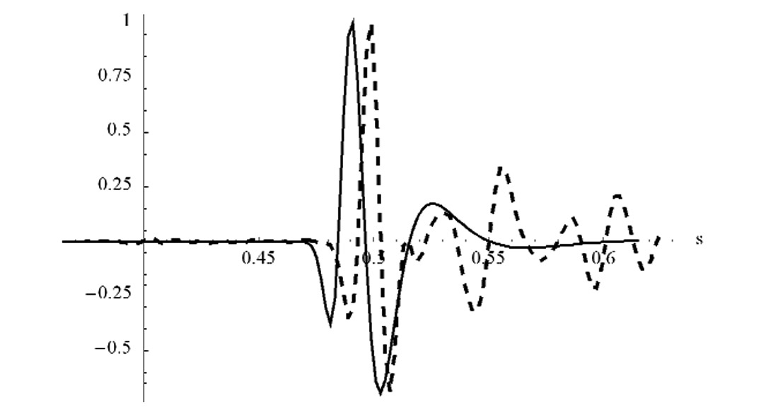
Figure 3 shows the MBWP model and the first arrival for a Vibroseis VSP experiment. Again a small time shift has been placed between the peak amplitudes to facilitate comparison of the waveforms.

Since the data and models match each other, this suggests that the MBWP procedure is able to model the seismic wavelet. If the data and model did not match each other, this would indicate that either the parameters associated with the MBWP model are incorrect or that there is some other filtering action in the seismic acquisition system that is not being modeled properly.

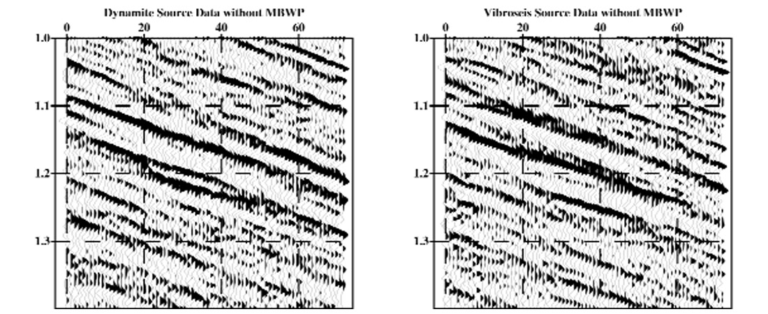
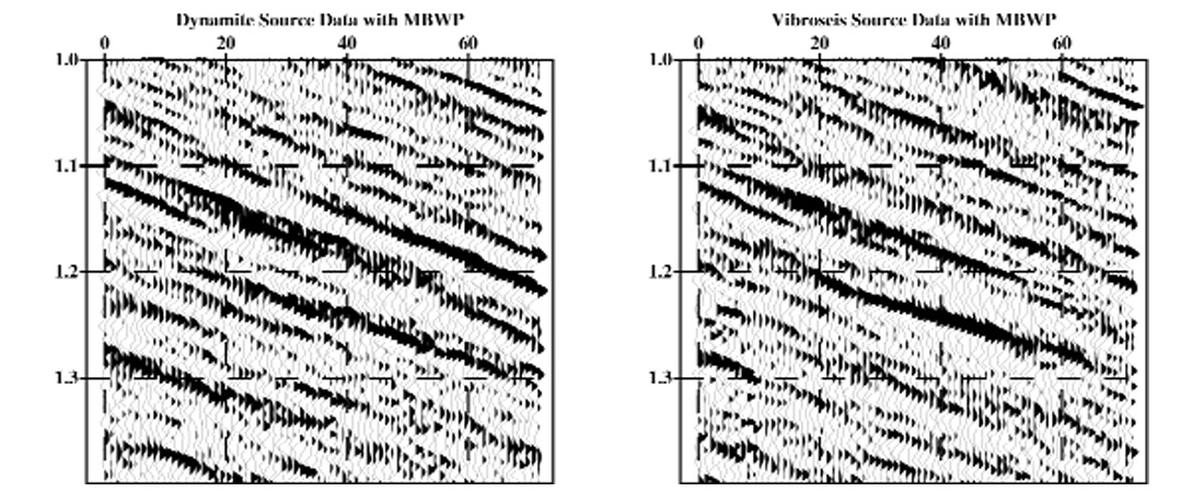
Another means that confirms the validity of MBWP, albeit more indirectly, is to design filters that correct both dynamite source data and Vibrosies source data to zero phase. Figure 4 is a comparison of dynamite source data and Vibroseis source data for the same CMP locations in a mixed-source 3D survey without application of the MBWP phase corrections. Figure 5 shows the same comparison after application of the MBWP residual filters.