A Tomostatics Primer

First arrival turning ray tomography is enjoying increasing popularity as a tool for deriving both weathering statics and near-surface velocity models for depth imaging. This tutorial-style article focuses on the former of these two applications, the so-called “tomostatics” algorithm. I’ll try to open up the tomostatics blackbox by providing insight into several questions, specifically:

• How does the algorithm work?
• Which data sets stand to benefit from its application? Which don’t?
• What are the key parameters, and what are good rules of thumb for their usage?

Although the following discussion is cast in terms of a comparison between 2-D tomostatics and the popular 2-D GLI refraction statics algorithm, the findings and insights should extend over to the 3-D case, and also to comparisons between tomostatics and any other layer-based refraction technique such as the time-term method.

Tomostatics theory (and a contrast with the GLI algorithm)

Tomostatics is an iterative algorithm which seeks to minimize the difference between observed and predicted first arrival travel times given some user-supplied initial model of the near surface. Although details in implementation will vary from program to program, the basic algorithm works as follows: The program first traces rays through the initial model, then sets up a system of linear equations relating the travel time residual vector (i.e., the misfit between observed and predicted travel times—the “knowns”) to the model update vector (the “unknowns”). The system of equations is solved to yield the model update vector, which is then added to the starting model to produce a new model. Rays are traced through this new current model and the process is repeated until the misfit becomes satisfyingly small. Once obtained, the final model is used to derive shot and receiver weathering statics in the usual way, by first computing the vertical travel time between shot/receiver location and the base of the velocity model, then subtracting this time from the travel time associated with vertical propagation between model base and datum elevation at a velocity equal to the replacement velocity.

If this sounds suspiciously like a description of the GLI approach to refraction statics, you’re following along to a tee, for both approaches employ the techniques of generalized linear inverse theory to invert first arrival picks in order to compute near-surface velocities (hence the “GLI” acronym). In fact, the only conceptual difference between tomostatics and GLI lies in the way the model is parameterized: in the former, the near-surface is typically divided up into a series of constant velocity rectangular cells and in the latter it’s divided up into a small number of vertically inhomogeneous layers where the velocity increases from layer to layer. For tomostatics, the actual model parameters are the slownesses within each cell, while for GLI, the model parameters are the layer thicknesses and velocities at each station. Subtle as this difference may seem, it has huge implications for the nature of the velocity models that each algorithm produces.

To explain the differing nature of the models produced by either approach, you first need to recognize that the model space for tomostatics is much bigger than for GLI. For example, consider a small 2-D line, say 150 shots, 120 channels, 300 stations. Assume that both algorithms use a horizontal sampling interval equal to the station spacing (a typical choice), and furthermore assume that the GLI analysis is based on the usual two-layer-over-a- halfspace assumption with a fixed velocity in the first layer (e.g., 610 m/s), while the tomostatics analysis is based on a velocity model of maximum depth 200 m with a (typical) vertical sampling of 2 m. The number of tomostatics unknowns (which is equal to the number of cells) is given by N_tomo = 300 * 200/2 = 30000. In the GLI case, where at each station there are four model parameters (two layer thicknesses plus the velocities in the second layer and in the halfspace), the number of unknowns is given by N_GLI = 4 * 300 = 1200. Note that in both cases, the number of knowns is equal to the number of first break picks (= 150 * 120 = 18000).

We’re now in a position to understand the intrinsic differences in velocity model character between the two algorithms. First off, it’s easy to see that by algorithm construction, the GLI approach produces a layered near-surface model. As for the tomostatics case, a primary factor influencing model character is the increase in “degrees of freedom” in the model space compared with GLI. Specifically, each small cell can assume an independent velocity, and the algorithm is not bound by the restrictive assumptions of layer-cake geology. While at first glance, this might seem to imply that the tomostatics algorithm is capable of reproducing whatever near-surface geology might be at hand, our optimism must be tempered by the fact that the tomostatics system of equations is inherently underconstrained (note there are fewer equations (18000) than unknowns (30000) in the above example). This system indeterminacy means that it’s necessary to impose constraints in order to stabilize the solution, and the introduction of constraints necessarily entails making some sort of a priori assumption about the nature of the data. Thus, while in principle the tomostatics algorithm is capable of reproducing any general near-surface velocity distribution, the practical reality is that the model character will ultimately be influenced by the choice of constraint type.

As for the question of whether tomostatics will produce a better result than GLI on any particular data set, the above discussion implies that the answer is probably ‘no’ if the true near-surface really is layer-based. In cases where the geology is not layer-like, the answer depends on whether or not the assumptions inherent in the constraints are compatible with the character of the true geology. For instance, the common practice of enforcing model smoothness by forcing the x- and z-deriviatives of the model update vector to be small (used in the present study) will probably give superior results to GLI if the near-surface geology exhibits gentle to moderate velocity gradients. However, this same constraint type may produce poor results in a near-surface environment featuring very short wavelength static pockets, where the velocity field exhibits large spatial derivatives even if the overall geological setting is non-layered.

Synthetic experiments

In this section I’ll examine three synthetic examples in order to illustrate the pros and cons of tomostatics in the light of the above theoretical discussion. In each of the three cases, I constructed a different simple near-surface velocity model inspired loosely by some real data experience. In order to make my experiments compatible with the assumptions inherent in any weathering statics computation, I forced the base of each velocity model to be laterally invariant. Sources and receivers were placed at a constant elevation, and 2-D finite-difference acoustic modeling was used to generate synthetic shot records with a maximum frequency of 50 Hz (such a low f_max was used to speed up computations) with shot and receiver spacings of 60 m and 20 m, respectively. Source-receiver offsets varied from example to example as indicated in the figure captions.

First break traveltimes were picked using a production algorithm and were used as input to the tomostatics algorithm. The tomographic inversion was performed using the smoothness constraints described in the previous section, with a constant gradient initial starting model and default production parameter settings (ten iterations were used in all three examples). Next, shot and receiver statics were computed using a datum equal to the recording surface and a replacement velocity equal to the velocity at the base of the true model. Finally, the same first break picks were input to an industry standard GLI-type algorithm, and the resulting static solution was computed and compared with both the tomostatic solution as well as the true static solution.

In order to avoid “dumbing down” the GLI runs, I experimented extensively with the GLI algorithm parameters (switching between two and three layer-over-a-halfspace models, changing the velocity of the weathering layer and experimenting with different amounts of smoothing). Interestingly, in spite of this considerable testing, I was unable to significantly improve over the results I obtained using workhorse parameters (two-layer-over-a-halfspace model, weathering layer velocity V_w = 610 m/s with default model smoothing).

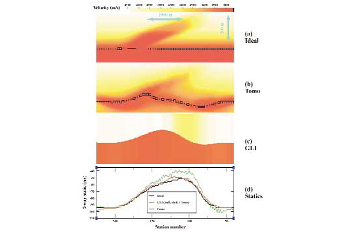
Example 1: overthrust model

Here the model consists of a single dipping lens of high velocity material (~4000 m/s, 5 degree dip) embedded in a laterally homogeneous background velocity field whose velocity varies relatively smoothly with depth (Figure 1a). Since this near surface model exhibits a significant departure from layer-cake geology, we expect that tomostatics should a better job than GLI. The near surface velocity model estimates from tomostatics and from GLI are shown in Figures 1b and 1c, respectively, and indeed they show that tomostatics has produced a better estimate of the velocity field, succeeding even in recovering some crude aspects of the velocity inversion (observed between stations 120 and 180). Predictably, the static corrections obtained from tomostatics are closer to the exact result than those obtained from GLI, especially in the vicinity of the inversion (Figure 1d).

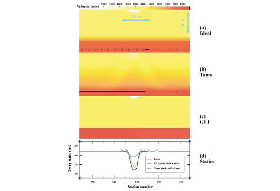
Example 2: shallow weathering pocket

In this example, a single low velocity weathering “pocket” (actually a Gaussian distribution with v_peak=1000 m/s, effective width=100 m, depth 30 m) is inserted into a laterally homogeneous layer-cake background model consisting of a 3000 m/s layer overlying a 4000 m/s halfspace (Figure 2a). The near surface velocity model estimates from tomostatics and from GLI are shown in Figures 2b and 2c, respectively (I chose V_w =1000 m/s for the GLI run, though I obtained equally good statics using V_w =610 m/s). Note that GLI has succeeded in correctly delineating the spatial extent of the pocket, and the associated statics correction (Figure 2d) is very similar to the true answer. On the other hand, the tomostatics algorithm has produced an “overly-smoothed” representation of the pocket, and consequently has underestimated the size of the static anomaly. Obviously in this case, the tomostatics smoothness constraints were not compatible with the character of the true model (which exhibits a relatively abrupt velocity change at the weathering pocket boundary). It’s worth noting that reducing the strength of the smoothness constraints, allowing the constraints to vary spatially, or employing a different type of constraint (e.g., edge-preserving) could help to improve the tomostatics result, but routine implementation is problematic for any of these alternative approaches. Clearly, the GLI algorithm is the natural choice in this layered near-surface environment.

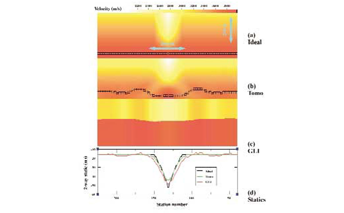
Example 3: smoothly varying low velocity anomaly

This example features a long wavelength (~ 800 m) low velocity anomaly which is embedded in a medium exhibiting gentle to moderate velocity variation in both x and z directions (Figure 3a). Given the gradient-like nature of this velocity distribution, it’s not surprising to see that tomostatics has recovered the true velocity model with good fidelity (Figure 3b) and produces a good statics solution (Figure 3d), nor is it surprising to observe that the GLI algorithm gives an erroneous velocity model estimate (Figure 3c).

Practical considerations

This section deals with various practical considerations associated with running the tomostatics algorithm.

Data-tying headaches

Given the potentially very different character of the models derived from tomostatics and GLI, it’s hardly surprising that the associated statics profiles are often bulk-shifted compared to one another (e.g., see Figure 1d). Since this bulk shift obviously implies a bulk shift in the final stacks, it can amount to a headache for an interpreter who is trying to tie different vintages of data.

Accuracy of travel time/ray tracing computations

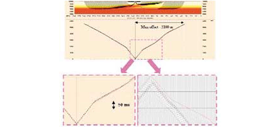
While the GLI algorithm can rely on analytic expressions for simple layered earth models in order to generate traveltimes and form its system of linear equations at each iteration, tomostatics must employ a more sophisticated travel time or ray tracing algorithm for these tasks. Accurate computation of traveltimes/ray paths in heterogeneous media is not a trivial business (a discussion of this topic is beyond the scope of this tutorial), but is nonetheless a necessary requirement for deriving accurate statics. Figure 4 displays the picked first breaks from a synthetic shot from Example 1, as well as travel times and rays computed by the tomostatics algorithm for the same velocity distribution. The agreement between picked first breaks and arrival times computed via the algorithm is very good (a good deal of the discrepancy is due to difficulties encountered in picking some of the weaker amplitude first breaks—see Figure 4, bottom right).

Computational expense

Run times are much shorter for GLI (often by more than two orders of magnitude), primarily because of the large computational expense associated with the travel time/ray tracing algorithm. An additional expense is incurred because the larger number of model parameters for tomostatics entails the inversion of a larger system of equations. Given these increased costs, clearly there is motivation to understand which classes of data sets stand to benefit most from application of tomostatics before running the algorithm!

Key run-time parameters

Although each algorithm will probably feature many user-codable parameters, I believe there are three main ones which can significantly affect the character of tomostatics result, as discussed below.

(i) choice of starting model

For better or for worse, it turns out that the tomostatics result depends to some degree on the choice of starting model. Using a smoothed version of the model from a previous GLI run as the initial model for tomostatics can be a good approach. However in cases where GLI has clearly failed and/or the geology is known to depart significantly from layer-cake, it may be advantageous to use a constant vertical gradient starting model (v=v0+kz). In such cases, it is a good idea to choose v0 and k such that the ray coverage associated with the initial model approximately coincides with the spatial extent of the true near surface model (which of course we never know with precision!).

(ii) base of model computation

The GLI model parameterization implicitly yields a very well–defined base of model (simply given by the base of the deepest layer). On the other hand, the determination of a base of model for tomostatics is a somewhat thorny task. In the above synthetic examples (e.g., Figure 1b), the base was set equal to the maximum depth of significant ray coverage at each station (this loosely corresponds to the maximum vertical extent of reliable solution determinacy). However, different algorithms may feature different strategies, (e.g., resolution matrix analysis, borrowing the base of drift from a GLI run, or keying on some deep isovelocity contour (Zhu et al., 2000)). Different approaches may lead to different static profiles and the optimal choice may depend on the data set at hand.

(iii) specification of constraint weights

Although the constraint schemes may vary from algorithm to algorithm, one common approach is to enforce model smoothness by defining an objective function of the form:

Φ(m) = misfit +μ₁ * size_of_x-derivative_of_m + μ₂ * size_of_z-derivative_of_m,

where m is the model update vector for a given iteration (by minimizing phi with respect to m, you obtain model parameters which tend to make the misfit and the derivative terms small at the same time; this produces a smooth model which fits the data well). The pressing question is: “how big do you make the scalars μ₁ and μ₂?”, and answering that question can be a tricky business. In the above examples, I chose μ₁ and μ₂ so that the power of the matrix associated with the constraint equations is in some sense close to the power of the matrix associated with the misfit equations. While theoretically this is not the correct thing to do, it seems to work well for the majority of cases, though it is still sometimes difficult to come up with an optimal choice without some experimentation.

Summary

Tomostatics employs a more flexible model parameterization than the layer-based refraction statics techniques, and consequently is capable in principle of modeling a broader class of near-surface environments. However this increase in model flexibility comes at the price of an increase in solution indeterminacy, and in practice the likelihood of obtaining improved statics estimates using tomostatics is directly related to the degree to which the assumptions behind the constraints are compatible with the real geology.

The conventional layer-based techniques still do a good job in a great number of cases (e.g. examples 2 and 3) from the viewpoint of the statics computation, if not necessarily from the viewpoint of the accuracy of the velocity model — and I think that the user should perform extensive parameter testing with the inexpensive conventional algorithm before arriving at the conclusion that tomostatics is producing the best results for any particular data area.

Having said that, there are some complex near-surface regimes out there which are completely incompatible with the layer-cake assumption, and in such cases tomostatics will probably give better statics (e.g. example 1). Moreover, in situations where the concept of statics breaks down, the more sophisticated approaches of either pre-stack wave equation datuming or prestack depth migration from surface are required to handle the near surface complexity, and the importance of getting a good velocity model becomes paramount (as opposed to just getting good statics like GLI does most of the time). For these reasons, I’m excited to see that tomostatics is beginning to occupy what I think is its rightful place in our production processing tool kit.

Acknowledgements

I’m grateful to Dave Aldridge, Andy Calvert, Scott Cheadle, Fuchang Guo, Oliver Kuhn and Brent Sato for helpful discussions. I’d also like to thank the Center for Wave Phenomena at Colorado School of Mines for use of their Seismic Unix finite-difference acoustic modeling software.