Abstract
In an unpublished CREWES report, Russell and Smith (2007) use measurements from Han (1986) to evaluate two different approaches to the modeling of Kdry versus porosity in clean sands: the pore space stiffness method and the critical porosity method. For the range of porosities found in the Han sandstones, Russell and Smith (2007) found that the pore space stiffness method gave a closer least-squares fit to the data than the critical porosity method. By performing fits over a range of different pressures, the authors were also able to derive a relationship between pressure and constant pore space stiffness, and hence between Kdry and porosity at different pressures or depths. In this study, I extend the work of Russell and Smith (2007) from the bulk modulus case to the shear modulus case and show that this will lead us to a new approach to the derivation of a rock physics template, or RPT (Ødegaard and Avseth, 2003), one that provides better agreement of the bulk to shear modulus ratio to published experimental studies (Murphy et al., 1993).
Introduction
In an unpublished CREWES report, Russell and Smith (2007) use measurements from Han (1986) to evaluate two different approaches to the modeling of Kdry versus porosity in clean sands: the pore space stiffness method and the critical porosity method. For the range of porosities found in the Han sandstones, Russell and Smith (2007) found that the pore space stiffness method gave a closer least-squares fit to the data than the critical porosity method. By performing fits over a range of different pressures, the authors were also able to derive a relationship between pressure and constant pore space stiffness, and hence between Kdry and porosity at different pressures or depths. In this study, I extend the work of Russell and Smith (2007) from the bulk modulus case to the shear modulus case and show that this will lead us to a new approach to the derivation of a rock physics template, or RPT (Ødegaard and Avseth, 2003), one that provides better agreement of the bulk to shear modulus ratio to published experimental studies (Murphy et al., 1993).
Pore Space Stiffness and the Gassmann Equations
Pressure plays an important role in rock physics. The compressibility of a porous rock, C, which is the inverse of the bulk modulus, can be written as the derivative of the volume of the rock with respect to pressure, divided by the volume itself, or

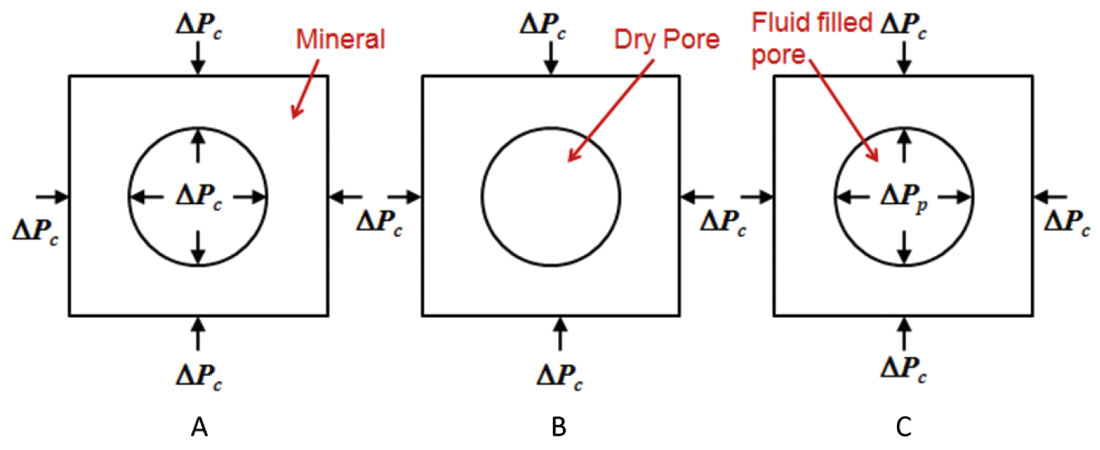
where V = volume and P = pressure. In equation 1, we are generally interested in two types of pressure: confining pressure, Pc, and pore pressure, Pp. Also, there are three different volumes to consider: the volume of the bulk rock, Vb, the mineral, Vm, and the pore space, Vp. Utilizing these concepts, we can build three simple models of the rock volume, and these are shown in Figure 1. In this figure, our rock model consists of the simplified case of a solid mineral with a single pore, where (a) is the situation where the confining pressure applied to the inside and outside of the mineral, and shows us that the rock deforms with the mineral modulus, (b) shows no stress on the inside of the rock but confining pressure on the outside, and therefore gives us the dry rock case, and (c) shows pore pressure on the inside and confining pressure on the outside, and gives us the saturated rock case.
The Betti-Rayleigh reciprocity theorem, originally published in the late 19th century, states:
“For an elastic body acted on by two different sets of forces, the work done by the first set of forces acting on the displacements caused by the second set of forces equals the work done by the second set of forces acting on the displacements caused by the first set of forces.” (Mavko and Mukerji, 1995).
As Mavko and Mukerji (1995) show in the appendix to their paper, if we use this theorem to first compare cases A and B from Figure 1, and then cases A and C, this will lead us to the Gassmann form of the Biot-Gassmann equation for bulk modulus. I will not reproduce the mathematical derivation from Mavko and Mukerji (1995) here, but simply state the results.
First, by comparing situations A and B (the mineral and dry cases), we arrive at the following equation:

where Kdry is the dry rock bulk modulus, Km is the mineral bulk modulus and Kϕ is the pore space stiffness.
The pore space stiffness is the inverse of the dry rock pore space compressibility, which can be expressed in the same form as equation 1 by

which states that the inverse of the pore space stiffness is equal to the ratio of the fractional change in pore volume to the full pore volume for an increment of applied confining pressure at constant pore pressure (Mavko and Mukerji, 1995). Note that this compressibility is identical to Cpc, (Zimmerman et al., 1986, Zimmerman, 1991) which is one of Zimmerman’s four fundamental compressibilities. In equation 2, I have used Zimmerman’s notation for pressure and also his sign notation. Mavko and Mukerji (1995) use different notation and also drop the negative sign.
Next, using the Rayleigh-Betti reciprocity theorem to compare cases A and C gives an equation involving Ksat, the saturated bulk modulus:

where
is the saturated pore space stiffness and Kf is the fluid bulk modulus. Notice the similarity between equations 2 and 4 and the fact that if the fluid bulk modulus is equal to zero, equation 4 simplifies to equation 2. We can re-express equation 2 as a function of pore space stiffness to get

Also, we can re-express equation 4 as a function of pore space stiffness to get

By equating equations 5 and 6 we can eliminate the pore space stiffness term, K. After dividing through by the mineral bulk modulus, Km, and the porosity, ϕ, and re-arranging the terms slightly, we then get

Equation 7 is one of the standard forms of the Gassmann equation (Mavko et al., 1998), and is used as the basis for fluid substitution. The fact that the Gassmann equation falls out so naturally from a derivation of the dry and saturated pore space stiffnesses suggests that these physical quantities are fundamental to the way in which porosity and pressure changes affect porous rocks in fluid substitution. This observation was tested empirically by Russell and Smith (2007), who used measurements from Han (1986) to evaluate two different approaches to the modeling of Kdry versus porosity in clean sands: the pore space stiffness method and the critical porosity method. A summary of their results will be given in the next section.
Pore Space Stiffness and Porosity
First, note that equation 2 can be re-arranged to give the following relationship

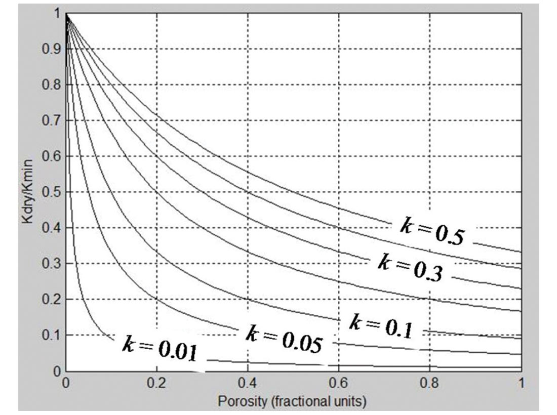
where k = Kϕ / Km. Equation 8 tells us that the dry rock over matrix bulk modulus ratio is an inverse function of porosity and the pore space stiffness over matrix bulk modulus ratio k. This equation confirms our observations that we expect this ratio to go to one at zero porosity. Also, it is clear that either as k gets smaller or ϕ gets larger, this ratio gets smaller, as shown in Figure 2.
The basic idea behind the pore stiffness method is that, for a given pressure, Kϕ should stay constant over a range of porosities, allowing us to re-compute Kdry at a different porosity. This will be discussed later in this section.
An alternate approach to changing Kdry as a function of porosity is the critical porosity method (Nur, 1992, Mavko and Mukerji, 1995), where the equation is given by

where ϕc is equal to critical porosity, which is the porosity that separates load-bearing sediments below ϕc from suspensions above ϕc.
The pore stiffness method and critical porosity methods represent two valid approaches to modeling Kdry as a function of porosity. Russell and Smith (2007) evaluated how well these two equations fit a dataset that was measured by De-hua Han for his Ph.D. thesis at Stanford University (Han, 1986). This dataset consisted of 70 separate sandstone samples of varying porosity and clay content (from clean to 51% clay). For each sample, measurements of P-wave velocity, S-wave velocity and density were done for both the wet and dry cases. In addition, the velocities were measured at pressures of 5, 10, 20, 30, 40 and 50 Mpa, respectively. This dataset was used initially by Han to predict the effects of porosity and clay content on the acoustic properties of sandstones (Han et al., 1986). In their discussion of the critical porosity method, Mavko and Mukerji (1995) used only the ten clean sandstones from Han’s dataset. From this subset of Han’s data, Mavko and Mukerji (1995) used all of the sandstones at 40 Mpa, which gave a reasonable visual fit to a critical porosity trend, and a single sandstone at pressures from 5 to 40 Mpa, which illustrated the fact that Kdry / Km is pressure dependent.
Russell and Smith (2007) performed an analytic study to determine which model gives the best fit to these points: critical porosity or constant pore space stiffness, in which they measured the root-mean-square error (RMSE) for the two fits, and also found the best values of k and ϕc. For the two fits they found, by using the ten clean sandstones at 40 Mpa pressure, that the RMSE for the pore space stiffness method was 0.039, and for the critical porosity method was 0.058. Thus, the critical porosity method gave a better fit to the points. For the pore space stiffness method the best fit value was k = Kϕ / Km= 0.162, and for the critical porosity method the best fit was ϕc = 0.343 (or 34.3%). The fits are shown in Figures 3(a) and (b).

Russell and Smith (2007) next performed a least squares fit to the full set of ten clean sandstones at each pressure: 5, 10, 20, 30, 40 and 50 Mpa. Their best fit values and RMS errors for each of the six pressure relationships is shown in Table 1. As can be seen in the table, the error is smaller for the pore space stiffness method in each case, and the values of pore space stiffness and critical porosity increase with increasing pressure, as we expect.
| P(MPa) | ϕc | RMSE | Kϕ / Km | RMSE |
|---|---|---|---|---|
| 5 | 0.289 | 0.126 | 0.104 | 0.094 |
| 10 | 0.311 | 0.107 | 0.129 | 0.076 |
| 20 | 0.329 | 0.079 | 0.147 | 0.055 |
| 30 | 0.338 | 0.069 | 0.156 | 0.044 |
| 40 | 0.343 | 0.058 | 0.162 | 0.039 |
| 50 | 0.348 | 0.053 | 0.166 | 0.038 |
| Table 1: The best fit values and RMS errors as a function of pressure for the critical porosity and pore space stiffness methods (from Russell and Smith, 2007). | ||||
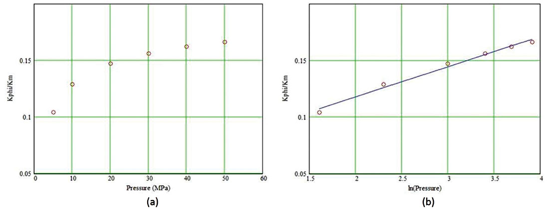
From the values computed for the pore space stiffness method, Russell and Smith (2007) then computed a relationship between pressure and Kϕ. Figure 4a shows the fit of Kϕ / Km versus pressure on a linear scale and Figure 4b shows the fit of Kϕ / Km versus pressure on a semi-logarithmic scale, where the natural logarithm of pressure has been plotted on the horizontal axis. The logarithmic fit is close to linear, and a best-fit linear fit was computed, with coefficients given by

Using calculus to differentiate equation 10, we get

Replacing the derivative with the difference operator and re-arranging, Russell and Smith (2007) then found that

Equation 12 is a useful result, since it allows us derive constant Kϕ curves at different pressures than the in-situ pressure, and hence predict a depth variable Kdry versus porosity relationship.
The Ødegaard / Avseth Rock Physics Template
Ødegaard and Avseth (2003) presented a new technique for the interpretation of elastic inversion results using what they called the rock physics template, or RPT, approach. In this method, they compute a theoretical template consisting of values of VP /VS ratio versus acoustic impedance (ρVP) and compare this template to results derived from both well logs and the inversion of prestack seismic data. To compute the values of velocity ratio and acoustic impedance, Ødegaard and Avseth (2003) compute Kdry and μdry as a function of porosity, ϕ using Hertz-Mindlin contact theory (Mindlin, 1949) and the lower Hashin-Shtrikman bound (Hashin and Shtrikman, 1963). The authors also incorporate the critical porosity method for the computation of the porous and solid phases. The bulk modulus computation is given as
and the shear modulus computation is given as

where HM is an abbreviation of Hertz-Mindlin,
P = effective pressure, Km and μm are the mineral bulk and shear moduli, n = the number of contacts per grain, Vm is the mineral Poisson’s ratio and ϕc is the high porosity end-member.
Once we have computed the dry rock bulk and shear moduli at different porosities, we can use the Gassmann equation (equation 7) to model the saturated rock properties. Gassmann’s theory predict that the shear modulus is independent of fluid content, or

The saturated density can be computed from the equation

where the subscripts m, w, g and o indicate matrix, water, gas and oil, S is the fraction of saturation of each fluid component. The only other term we need to know in equation 7 is Kfl, the fluid bulk modulus. This can be computed by the Reuss average given by

(Note that this is for uniform distribution of the fluids. For patchy saturation we use the linear Voigt average).
We can then compute each new saturation value by re-arranging equation 7 to give

where

and varying the value of Sw and ϕ.
Finally, we plug the new values of the bulk and shear moduli and the density into the equations for P and S-wave velocity in the saturated, porous reservoir, given by

and

From equations 19 and 20 we can finally compute the VP /VS ratio and the P-impedance, which is the product of density and P-wave velocity.
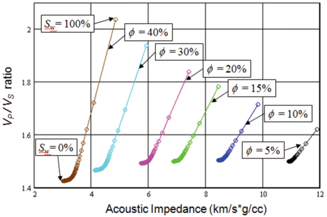
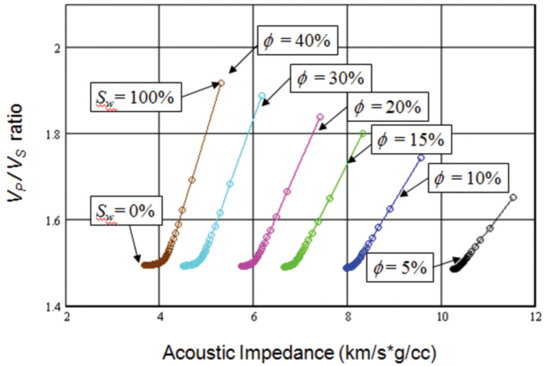
Figure 5 shows the computation of a set of curves in which we varied porosity and saturation using the following parameters: Km = 36.8 GPa and μm = 44 GPa (which implies that nm = 0.073), n = 8.64, and P = 0.02 GPa. For the saturation change we assumed a two phase gas-water system in which Kwater = 2.92 GPa and Kgas = 0.021 GPa. For the density, we assumed that ρm = 2.65 g/cc, ρwater = 1.09 g/cc and ρgas = 0.001 g/cc.
A Gassmann-Consistent Rock Physics Template
In this section, we will derive a new rock physics template based on the pore space stiffness approach. As shown by Russell and Smith (2007), equation 2 allows us to model Kdry at different porosities. To do this, note first that equation 2 can be re-written as

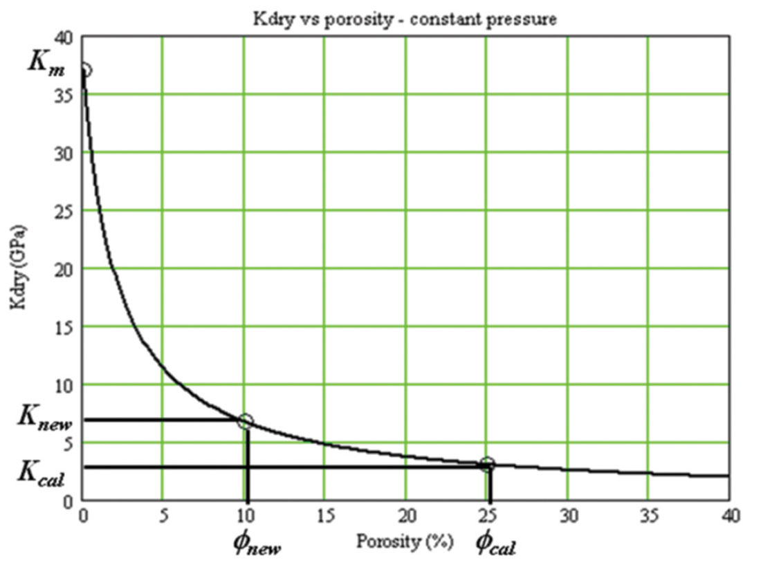
Thus, if Kdry is computed at some known porosity Kcal, where the subscript cal stands for calibration value, we can derive the value of Kϕ in the following way

Assuming that the pore pressure stays constant, a new value of dry rock bulk modulus Kdry_new new at a new porosity new will have the same pore space stiffness. That is, we can write

Combining equations 22 and 23, we can eliminate Kϕ and compute the new value of the dry rock bulk modulus as follows:

This is shown in Figure 6, where it is clear that we simply move along the curve of constant Kϕ.
Finally, we need to compute the shear modulus as a function of porosity. As shown empirically by Murphy et al. (1993), the modulus ratio Kdry / μ is remarkably constant for clean sandstones over a range of porosities. The authors found a value of 0.9 for this ratio. Assuming that this ratio is constant, regardless of its value, once we have computed the in-situ and new values of Kdry, we can compute a new value for the shear modulus by the equation

Although the use of equation 25 would seem reasonable, it has one major limitation. This is that the value of the shear modulus will generally not give the correct value at the mineral limit, unless the ratio at this limit happens to be the same as the ratio at the calibration point. For that reason, we decided to use an equation which is identical in form to equation 24, or

Figure 7 shows the results of applying equations 24 and 26 to compute porosity change from 5 to 40% and the standard Gassmann approach, described in the previous section, to compute saturation change from 100% wet to 100% gas (Sw = 0%). All of the parameters used in Figure 7 were the same as for the Ødegaard and Avseth method except that, since we are not using the Hertz-Mindlin approach, we did not need the coordination number n or the pressure P. Note that the absolute pressure does not enter our new approach, only the relative pressure change using equation 10. In this case, the pressure does not change, so we have no need to use this equation. However, we still needed to calibrate the two sets of curves. To do this, we used the value of Kdry computed for the 20% porosity case using the Hertz- Mindlin approach. This ensures that the results of the two methods will be identical for a porosity of 20%.
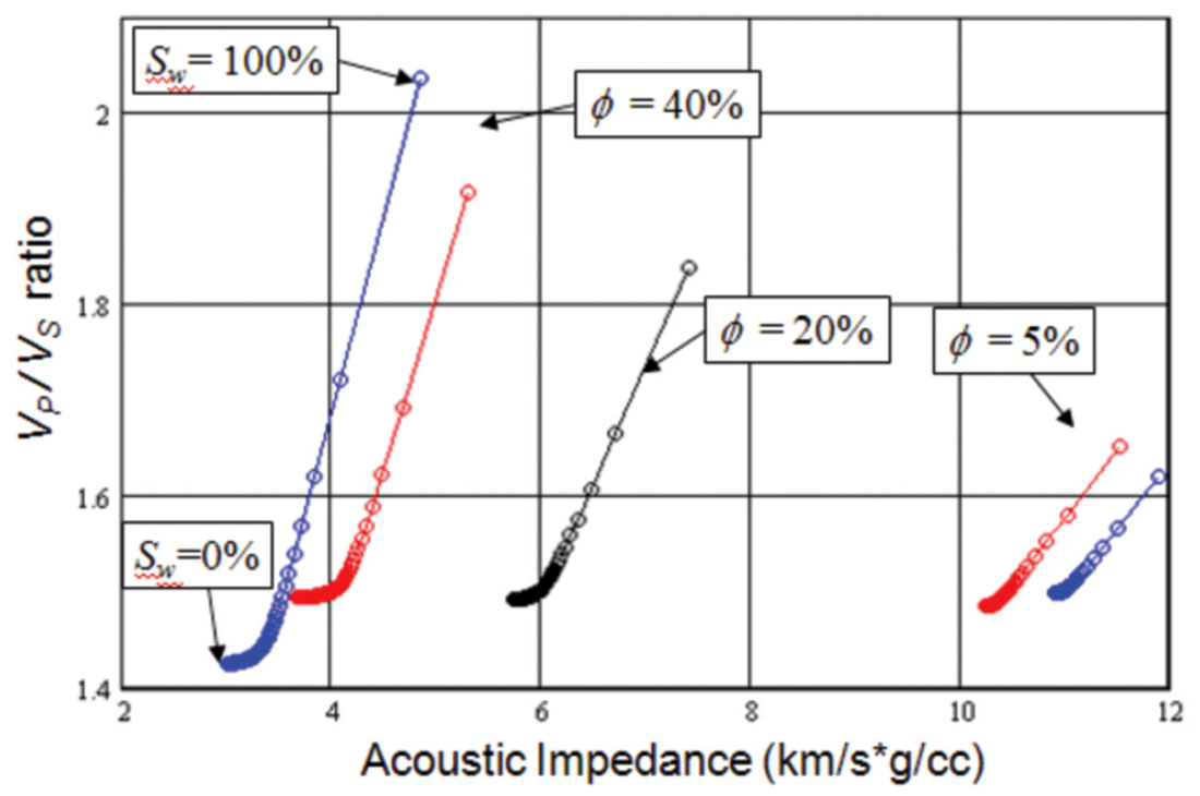
A comparison between the results in Figures 5 and 7 is shown in Figure 8, where we have displayed on the results for porosities of 5%, 20% and 40%. In Figure 8 notice that, as expected because of the calibration, the results of the two methods are identical at 20% porosity. However, at the extreme values of 5 and 40%, the pore space stiffness method appears to be “squeezed” in acoustic impedance compared to the Hertz-Mindlin method. That is, at a porosity of 40%, the Hertz-Mindlin approach gives a greater acoustic impedance value than the pore space stiffness method but, at a porosity of 5%, the Hertz-Mindlin approach gives a smaller acoustic impedance value than the pore space stiffness method. However, for the P to S-wave velocity ratio, the situation is different, and the Hertz-Mindlin approach gives a larger range of values at 40% whereas the pore space stiffness method gives a larger range of values at 5%.
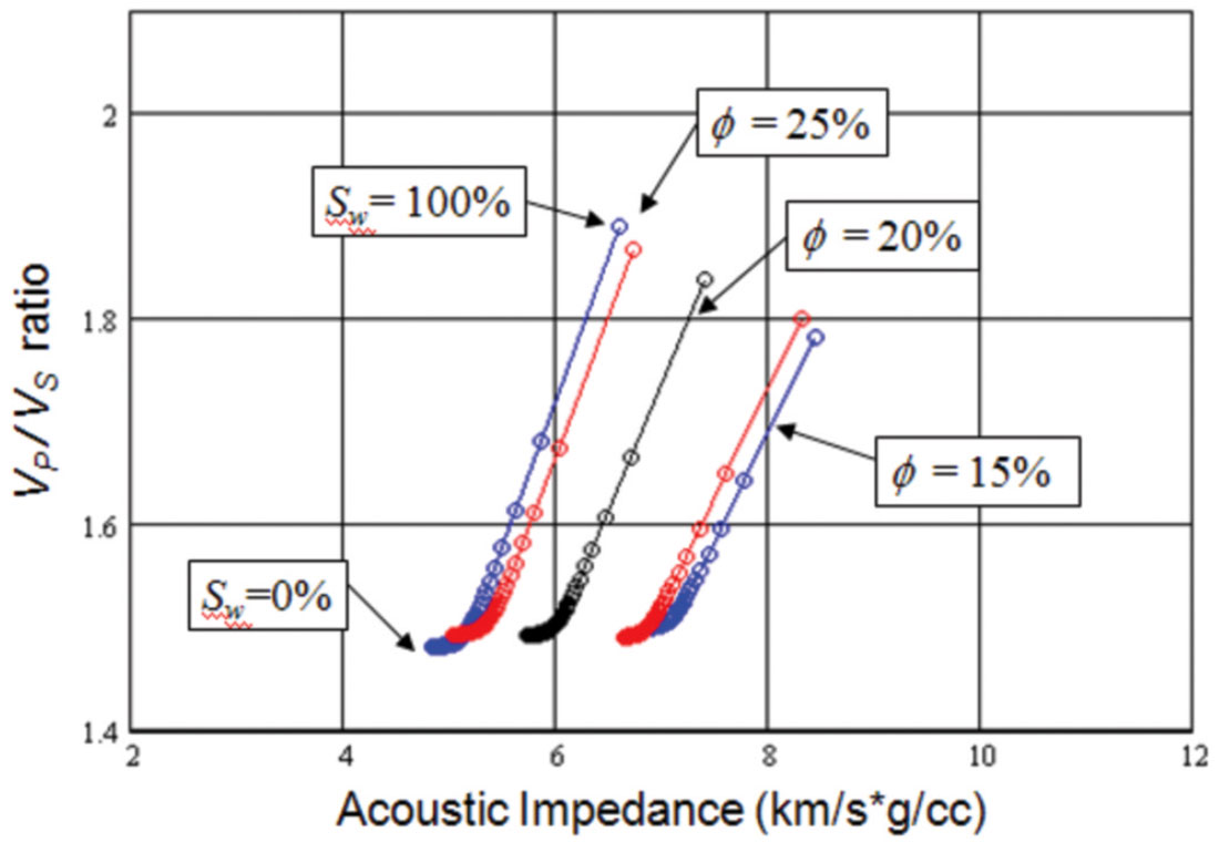
However, doing the computations over such a large range of values of porosity as shown in Figures 7 and 8 is probably pushing both methods too far. Thus, Figure 9 shows the comparison of the two methods over a range of 10% (plus and minus 5% from the calibration value). Notice that the discrepancies between the two methods are now much less.
Of course, the key question is: which of the two methods is correct? In fact, the real question is: which of the two methods is closer to being correct, since of course both methods are much too simplistic to exactly predict the behavior of complex earth materials. The ultimate test is to compare these templates with real data, both from well logs and seismic inversions. However, even here we might be in doubt as to which method works best, because the results will be dependent on how the scaling is done.
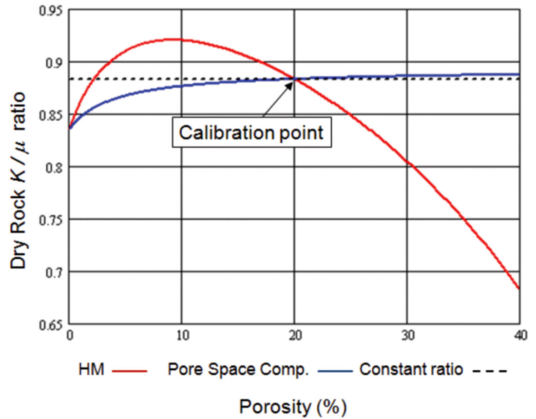
Therefore, to test the accuracy of the two methods, we used published experimental data. As mentioned earlier, it was shown empirically by Murphy et al. (1993) that the modulus ratio Kdry / μ is remarkably constant for clean sandstones over a range of porosities. The authors found a value of 0.9 for this ratio. Therefore, a good test of the two methods is to plot the Kdry / μ ratio found using these calculations. This is shown in Figure 10, where the constant dashed line is equal to the dry modulus ratio found at the calibration porosity of 20%, a value of 0.884. The red line is the ratio found by the Hertz-Minlin (HM) method, and the blue line is the ratio found using the pore space compressibility (PS) method. Note that the HM and PS lines intersect twice, once at the calibration point and once at the mineral (0% porosity) point, a value of 0.884 (the fact that this value is close to Murphy et al.’s value of 0.9 shows that, at the calibration point, the HM method is quite good). However, note that the HM line significantly deviates from the expected constant line, whereas the PS line is quite close except where it is forced to deviate to produce the fit at 0% porosity.
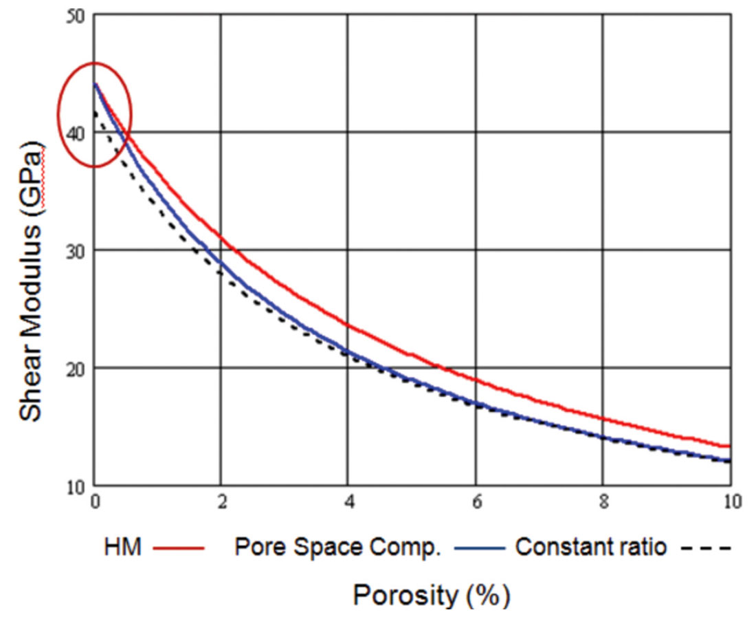
To make this clearer, I next plot the actual shear modulus curve as a function of porosity. In Figure 11, we plot this curve over the full range of porosities, from 0 to 40%, and in Figure 12 we plot only the porosities from 0 to 10%. In both plots three different models are shown: the Hertz-Mindlin approach, the pore space compressibility approach, and the constant ratio approach. Based on the measurements made by Murphy et al. (1993), we would expect that the constant ratio approach should produce a shear modulus which is most physically realistic, except for the zero porosity mineral case.
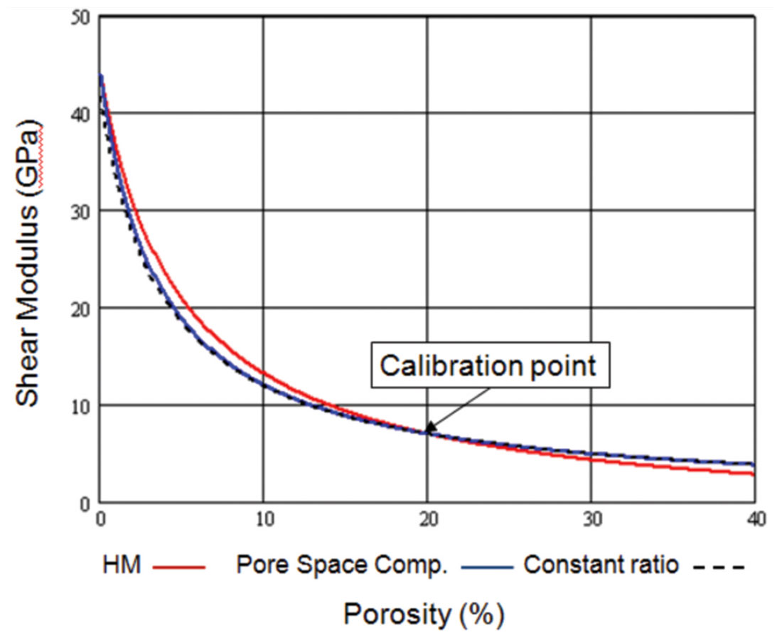
In Figure 11, it is obvious that the three curves all tie at the calibration point, as they should. However, over most of the range of porosities, the shear modulus computed using pore space compressibility approach ties the shear modulus from the constant ratio approach.
Due to the large range of porosities plotted in Figure 11, it is difficult to see what happens close to zero porosity. To illustrate this region, we have therefore plotted only the porosities from 0 to 10% in Figure 12. Note from this plot that, as we get arrive at 0% porosity (shown by the red ellipse) the Hertz-Mindlin and pore space compressibility approaches give the correct value for μm of 44 Gpa, whereas the constant ratio approach underestimates this value.
Based on the results shown in Figures 11 and 12, we therefore conclude that the pore space compressibility approach combines the best features of both the constant ratio approach, where the dry modulus ratio is constant for most porosities, and the Hertz- Mindlin approach, where the correct value of the mineral shear modulus is predicted at zero porosity.
Real Data Examples
Finally, I will apply this new rock physics template to a real dataset. But first I will display an interpretation of the trends found in a rock physics template. Figure 13, from Ødegaard and Avseth (2003) shows that we can interpret the various clusters on a rock physics template in terms of their mineralogy, fluid content, cementation, pressure and clay content.
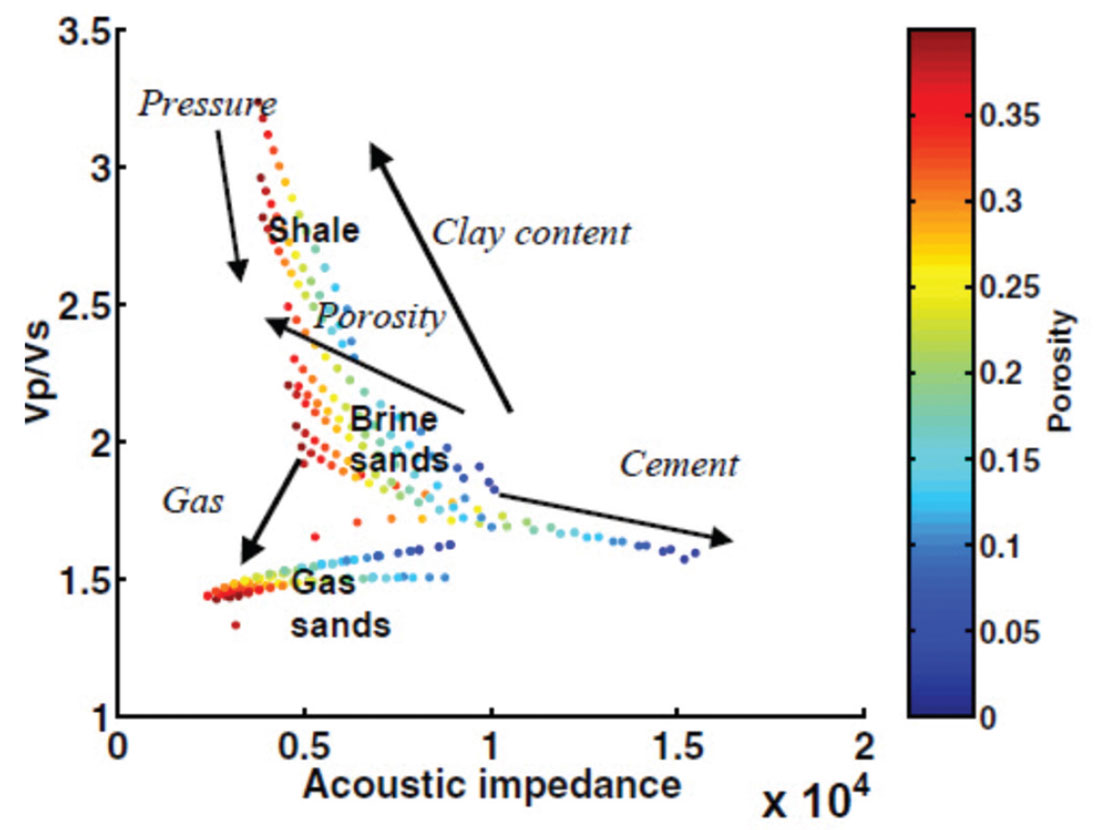
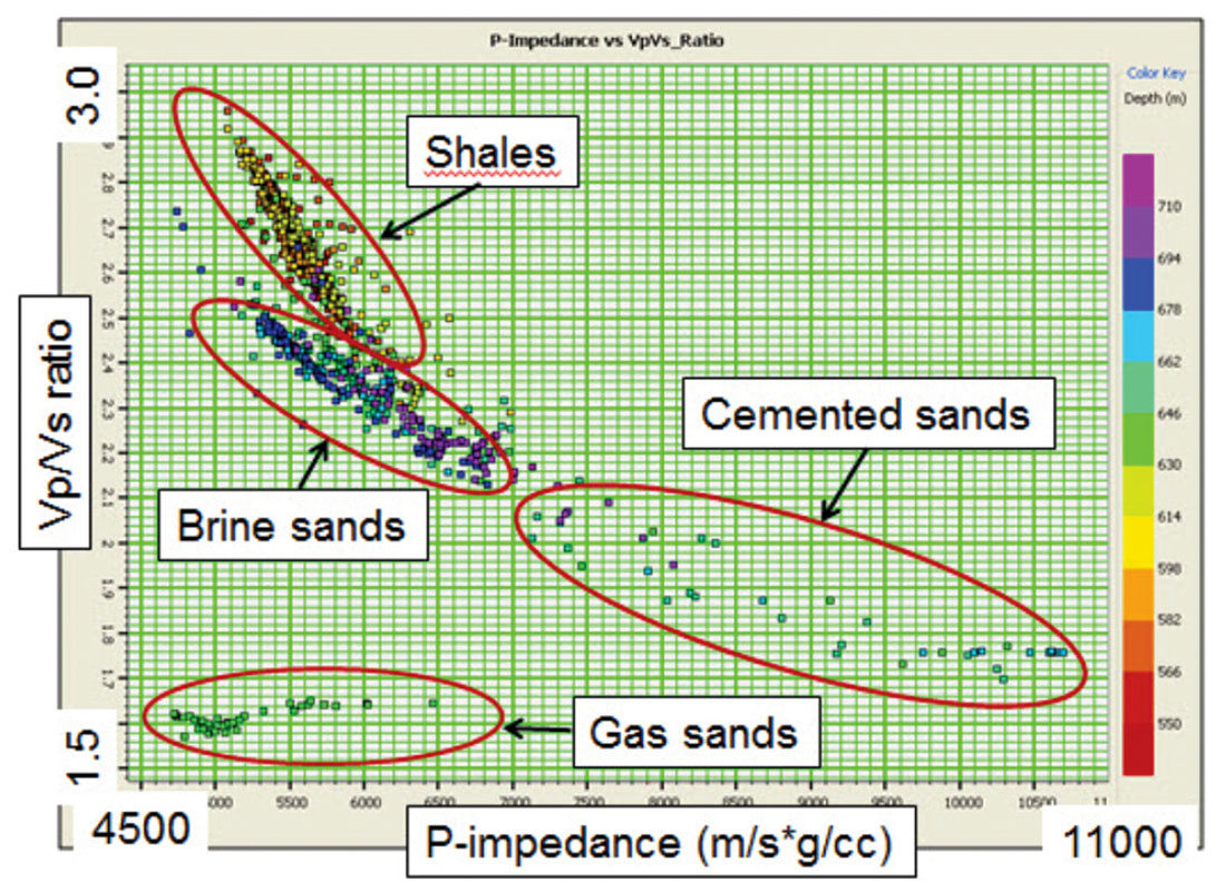
Now we will compare measured well log and seismic data to both of our templates and also to the interpretation of the templates shown in Figure 13. Figure 14 shows a crossplot between VP /VS ratio and P-impedance from well log data taken from a gas sand play in the Colony area of Alberta. The Vp (sonic) and ρ (density) logs were measured and the VS (dipole sonic) log was computed using the mud-rock line over the shales and wet sands and the Gassmann equations in the gas sands. The colour scale shows depth in metres. The elliptical regions on the plot show the various trends that were indicated in Figure 13, and have been interpreted from the well logs to correspond to these fluid and lithology units. Note the excellent tie between the interpreted clusters and trends in Figures 13 and 14.

The results of a simultaneous pre-stack inversion from the same area are shown in Figure 15. In this figure, we have cross-plotted VP /VS ratio versus P-impedance over the gas sand zone of interest, where the VP /VSratio was derived by dividing the inverted P-impedance by the inverted S-impedance. The colour scale is seismic two-way time in msec. Note that the range of values is less extreme than on the log data due to the bandlimited nature of the seismic data. However, the interpreted events again correlate extremely well with the trends and clusters shown on Figure 13.
Finally, I show the log and seismic data superimposed on the two different rock physics templates, where the log data has been integrated to time. Figure 16 shows the points from both the log data and seismic data superimposed on the same plot, where the red squares show the time-integrated well log data and the black squares show the inverted seismic results. On this plot, we have also superimposed the Ødegaard and Avseth template. The gas sand and wet sand values plot where we would expect on the template and the range of porosities between 20 and 30% are what are expected from the well log data. The fact that there are a large number of well log and seismic inversion values that plot higher than the limit shown on the template is due to the fact that these are shales, and the template was designed for clean sands.
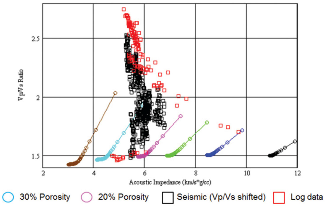
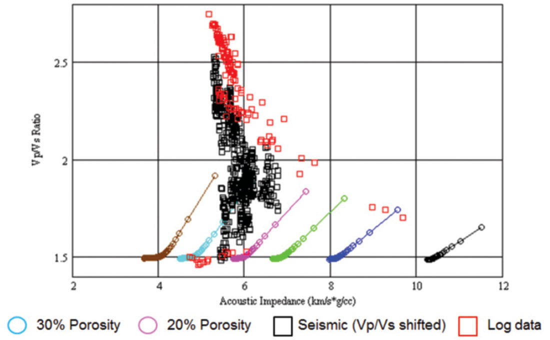
Figure 17 again shows the points from both the log data and seismic data superimposed on the same plot, where the red squares show the time-integrated well log data and the black squares show the inverted seismic results. On this plot, we have now superimposed the Gassmann template. As with the previous template shown in Figure 16, the gas sand and wet sand values plot where we would expect on the template and the range of porosities between 20 and 30% are what are expected from the well log data. The large number of well log and seismic inversion values that plot higher than the limit shown on the template is again due to the fact that these are shales, and the Gassmann template was designed for clean sands.
Based on the results shown in Figures 14 through 17, in which both well log and seismic inverted results have been compared to the two templates discussed in this paper, it would appear that both templates fit the results from both gas and wet sandstones very well. Either template could therefore be used successfully in a real exploration play. However, based on the considerations discussed in the previous sections, there is a fundamental simplicity implied in the Gassmann template that makes it easier to understand and interpret, especially in terms of standard poroelasticity theory.
Conclusions
In this study, I have discussed a new approach to the derivation of the rock physics template, or RPT, and compared this new approach to a previously published approach (Ødegaard and Avseth, 2003). I first discussed pore space stiffness and used the Betti-Rayleigh reciprocity theorem to derive Gassmann’s equation from the dry and saturated pore space stiffnesses, as suggested by Mavko and Mukerji (1995). From this very intuitive approach to the derivation of the Gassmann equation, it was clear that pore space stiffness plays a very important role in the understanding of the way that dry rock bulk modulus changes as a function of porosity for constant pore pressure. I then reviewed the empirical work done in CREWES report by Russell and Smith (2007) to show that the pore space method does indeed give a good fit to measured sandstone values by Han (1986).
After reviewing the work of Ødegaard and Avseth (2003), which was based on Hertz-Mindlin contact theory, the lower Hashin- Shtrikman bound and the critical porosity method for the computation of the porous and solid phases, I then discussed how to use both the pore space stiffness and Gassmann equations for estimating bulk and shear modulii as a function of saturation and porosity to build a similar type of rock physics template. Using empirical measurements in sandstones, I next compared the two approaches. I showed that this new method is both more intuitive and also produces a dry modulus ratio as a function of porosity which is closer to that derived in experimental studies of Murphy et al. (1993). Finally, I used a measured set of well log values and the associated pre-stack seismic inversion values to test these two template approaches in a real exploration play. Both templates gave reasonably good fits to the measured well log and seismic data. However, based on the considerations given earlier in this study, the Gassmann template provides a simpler, more intuitive interpretation of the data, one that is based entirely within poroelasticity theory. In summary, this new method is more appealing from the point of view of Occam’s razor, or the law of parsimony, which states that “simpler explanations are, other things being equal, generally better than more complex ones.” (from Wikipedia, the free encyclopedia).


Join the Conversation
Interested in starting, or contributing to a conversation about an article or issue of the RECORDER? Join our CSEG LinkedIn Group.
Share This Article