3D Seismic Surveys – Past, Present and Future

Overviews are often useful and this paper is written for the geophysicist who has not been deeply involved with the design and analysis of 3D seismic survey acquisition for the past 15 years or so, and would like to have an idea of what happened, what’s happening now and what is likely to happen in the future.

Past

It began as early as 1964 when Hugh Hardy of Esso shot the world’s first cross-spread - before it even had a name! By the 70’s it became a search for better, more accurate signal. Our understanding of 2D seismic surveys - their acquisition, processing and interpretation - was extremely comprehensive. Even back then, some said it was complete - at least for the purpose of finding oil and gas. But the language of the day still contained some disturbing phrases such as “Sideswipe” or “Out of the Plane”. The answer was 3D.

Early efforts began with areal distributions of sources and receivers in an attempt to create continuous areal CMP coverage. A good example was a method called “Seisloop” by GSI where shots and receivers were placed in contiguous loops (as, for example, around the edges of a field). The final CMP coverage extended from the edges of the loops to their center.

In 1978, a 3D survey was acquired near Calgary using orthogonal shot lines and receiver lines. As a programmer then, it was my task to build methods to process this data set. The main pieces of the puzzle involved modifying the existing 2D crooked line geometry software to handle the new concept of 3D CMP bins - and a new program to display time slices. Time slice displays were just appearing in the literature at the time and none of us involved in the project had any good idea of what these new displays might show. Imagine the excitement as the display was unrolled and we walked down the corridor (and down in time) inspecting each slice as we went. We marveled as reef tops appeared out of nowhere and literally seemed to grow out of the floor as we walked. We were sold!

In the early 80’s orthogonal geometries were the norm. It seemed as if this was the only way to shoot 3D - and clearly more logical (and easier logistically) than the earlier attempts. 3D migration software was written and targets became more focused than they had ever been. The problem was solved and confidence in the new exploration technology increased by leaps and bounds. Predictions as to the demise of 2D were everywhere.

Then, many of us noticed the noise. Starting in the late 80’s and early 90’s it became obvious that a lot of the 3D surveys contained more noise than signal - or, at least, more noise than previous 2D. So the quest to kill the noise began.

Geometry was the weapon of choice. It became clear fairly quickly that the best way to attack noise was through the act of CMP stacking. Offset and, to a lesser extent, azimuth distribution was recognized as the most important factor. In other words, the various offset traces that “belonged” to each CMP bin contained different levels of noise and the act of CMP stacking attenuated the noise. The new geometry weapon was therefore aimed at improving the offset distribution.

The ever-fertile geophysical minds of the day created geometry after geometry in rapid succession. A partial list (who can remember them all?) reads like this:

Orthogonal

This tried and true method persisted throughout.

Indents

Moving shot and receiver lines one half ( or quarter, etc.) station intervals. The term “Odds and Evens” was sometimes applied to such geometries.

Staggered line recording

This term was used when the indents were arranged to create CMP bin scatter (spread the midpoints in each CMP bin to achieve sub-bin sampling).

Brick

The Brick was first invented to improve the offsets. Later it was realized that the largest minimum offset was also reduced.

45 degree lines

Contractors quickly tired of trying to shoot bricks through trees, so the slanted geometries were born.

Slanted bricks

These were often referred to as drunken bricks (the terminology is clearly unrelated to the inventors!)

Triple bricks

If two is good, three must be better?

Button patch

Invented, used (and patented) by ARCO only.

The 4 line patch

Progenitor of the wide vs. narrow debate. The 4 line patch was only a few hundreds of metres wide - and very long - and cheap! Many articles were written extolling its virtues as the only 3D geometry you would ever need.

The wide line patch

The other side of the debate. An equal number of articles extolling the virtues of the wide patch were written. Who was right? The quick answer is that time has favored the wide patch - mostly because of better offset distribution for noise attenuation and generally reduced artifacts due to the wide sampling. However, many narrow patch surveys are still conducted.

Flexi-Bin

Invented and patented by GEDCO. Sub-bin sampling seemed to be attainable with this method, which involved non-integral line spacing with respect to station spacing. The passage of time has proved that sub-bin sampling cannot be achieved by this or other such methods (like indents and staggered line recording), but the geometry has turned out to have other (considerable) advantages over the standard orthogonal geometry (e.g. improved offsets and statics coupling and, based on practitioners’ experiences, improved interpretability).

Megabin

Invented and patented by PanCanadian. This method was an attempt to use a viable subset of the fully sampled 3D geometry. (All 3D’s are decimations of the fully sampled 3D that has shots and receivers everywhere on a grid). Indications are that linear shot noise, backscatter and multiple energy are well attenuated by this geometry - perhaps better than by orthogonal. Sub-surface sampling tends to be coarse (70 x 35m bins are fairly routine) and FX interpolation is normally used to create in-fill traces prior to migration.

26 degree lines

First appearing from Amoco’s Tulsa research, this geometry appeared to improve offset distribution considerably. “Footprints” were much reduced and this became (and still is) a very popular choice in the war against noise.

Zigzags

In desert areas, this method allowed vibrators to travel a zigzag path between two adjacent receiver lines without crossing them. Logistically it was a very attractive, cheap method to acquire data in such areas. Good access is essential.

Double zigzags

The big disadvantage of the single zigzag was very poor noise attenuation. It was rumored to be the geometry with the biggest footprint of all. The double zigzag cured that and is still a popular geometry in desert regions.

Triple zigzags

Once again if two is good, three must be better. Logistically this is very attractive - 50% less receiver effort (increase the line spacing) for the price of adding a third vibrator crew. Practically it seems to be producing acceptable data.

Full swath rolls

Logistically very attractive - shoot along the width of a survey using a salvo of shots extending outside a narrow patch at each shot line, thus achieving wide azimuth and offset distribution, then roll the entire patch up and go back across the survey. The only real disadvantage is the minimal statics coupling between swaths (shots only). Each shot is fired twice (or more depending on the salvo width). Thus it is possible to have different shot statics at each shot position because of differing ray paths.

Sparse 3D

Wide line spacing is the norm - up to one kilometer or more between shot and receiver lines. The idea is to cover a large area with 3D and do it in the most cost-effective manner. Unfortunately such 3D’s have high noise content and can be difficult to interpret.

Dense 3D

Very tight shot and receiver line spacing is the norm here. Extremely high fold is also common. Data quality can often be better than conventional 3D’s by an order of magnitude. Expensive but very interpretable!

18 degree lines

The final chapter (so far!) in the slanted line progression. The current thinking is that 18 beats 26 which beats 45. Time will tell!

Random

When everything else had been tried, random positioning of shots and receivers was left. Many random 3D surveys have now been conducted and the results indicate that this method does have considerable merit in reducing the seemingly ubiquitous footprint suffered by other geometries. Imaging is often done using pre-stack time migration and results appear comparable to other geometries. Significant cost savings can also be realized.

In the 90’s geophysics came to grips with this plethora of geometries. Science and sampling theory were applied and everyone came to realize that 3D’s were badly under-sampled. Could they ever be made to fit the budget?

As the millennium approached, the effort to seek signal was almost equal to the effort to nullify noise. The various types of noise were, by now, well recognized and a body of knowledge grew as to what worked on each of them. Here is a brief list:

Linear shot noise

This includes air blast, ground roll and other near surface waves traveling horizontally from shot to receiver.

Backscattered shot noise

Near surface scatterers can cause each of the linear noise waves to be reflected. Thus the waves travel by a path from shot to scatterer to receiver. Backscatter can often be the single largest noise component in recorded seismic data.

Multiple energy

Surface and interbedded.

3D Statics

Delays in travel times caused by near (or even far) surface anomalies can be a source of noise. The simple perspective is that if such static delays cannot be removed they will diminish the signal content. 3D geometries differ in their ability to resolve 3D static delays.

The nature of offset distribution and azimuth distribution and how they change with depth became crucial in studying the noise problem.

During this time there was also discussion about apertures - both the aperture recorded by single shots and that of entire surveys. Some conclusions were clear. First that resolution varied throughout a survey - becoming larger near the edges and near the end of recording time ( in this context, larger resolution means less ability to distinguish two adjacent sub-surface features). Second that the size of a bin can determine resolution because of anti-alias criteria. Thus large bins set the limit on resolution and therefore on the maximum useful frequency. To put it another way, additional high frequencies have no effect on resolution when it is set by the bin size.

The debate about combining individual shots - or components of shots (e.g. offsets) to form a complete pre-stack time migrated volume is the subject of much current work. Vermeer (SEG Convention, 2000) showed how common offset vector tiles (formed from symmetrically sampled orthogonal geometry) could be used to create a continuous migrated volume with minimal “edges”. The answer to the same question for other geometries is still unresolved.

Also during the late 80’s and much of the 90’s processing started to catch up on acquisition. Rapid progress was made in understanding the algorithms needed for:

• 3D surface consistent scaling and deconvolution.
• 3D refraction statics.
• 3D residual statics..
• 3D linear noise removal (FK, Tau-P, Radial trace and many others).

On the question of noise attenuation, the jury is still out. New processing algorithms often appear to make a substantial difference to individual shots (or receiver line components of shots). But the CMP stacks with and without the noise removal algorithm often look distressingly similar, leading to the conclusion that CMP stacking is still the best weapon in the anti-noise armory.

Imaging in the early days was all done post stack - typically through 3D Kirchhoff or FK migration. Later, other post-stack methods were added to the arsenal - Finite Difference, Phase Shift and other more exotic variants. Post stack depth migration has also made an appearance in the past few years.

In the pre-stack domain, DMO was the algorithm of choice for many years (and still is in many parts of the world). Recently many practitioners have noted that geometry can dramatically affect the output of DMO. In particular, wide towed marine streamer data (multi-source, multi-streamer) after DMO had a very striped appearance. This was also predictable from theory and has been remarked on by a number of authors.

In the past few years there has been a decline in the use of DMO and an increasing emphasis on pre-stack time migration.

Present

The number one question on everybody’s lips today is, “What’s the best geometry for my 3D?” The number one answer is, “It depends!”

Is signal the goal? In this case, the best sampling method that can be reassembled into the various spatial wavelengths in X, Y and Z must be chosen. G. Vermeer has written the book on this approach and it involves symmetric sampling - whatever is done to shots must also be done for receivers. Equal sampling everywhere - stations, lines and even the survey size if possible! By using symmetric sampling, the most focused image can be guaranteed. (Note that the absolute best answer is to use the fully sampled 3D geometry - this is the one design that will always exceed the budget.)

Or is noise attenuation more important than signal? It is often the case that noise must be reduced before signal can even be seen. Today’s best geometries for noise attenuation seem to be wide azimuth slanted geometries with 18 degrees often emerging as the winning angle. The small departure from orthogonal (18 degrees instead of zero) does not dramatically affect the imaging properties either. Double or triple zigzags can work well against linear noise, but the imaging (migration) can have more “edges” than an orthogonal geometry and therefore appear less focused.

On the question of reducing multiples, this is the most active area of research today. The only consensus so far in this debate is that wide azimuth surveys will be better than narrow - simply because of the preponderance of long offsets and the offset-squared distribution. Other factors like unequal shot and receiver line spacing and slanted lines are currently under investigation.

To coin a phrase, today’s geometries are Designer geometries!

In other words the geometry that is best suited is the one that best addresses the specific local problems of improving signal at a chosen target, while identifying and reducing the various sources of noise.

Arrays are also making a comeback. Since 2D gave way to 3D, arrays have been largely ignored. All too often bunched phones and single holes have been the norm. Recently many acquisition geophysicists have made attempts to reduce linear and backscatter noise before it reaches the recorder. While there is no shortage of anecdotal knowledge, there is still a lack of broadly based experiential knowledge about the use of arrays in 3D. It is worth remembering that if shot noise can be reduced by 6dB using a better array, this is equivalent to quadrupling the CMP stack fold!

In a similar vein, it is also worth remembering that if the CMP stack for one geometry attenuates the noise by 6dB when compared to the CMP stack for another geometry, the fold has again been effectively quadrupled.

Future

Time-lapse 3D recording is becoming more widely used. So one of the first immediate challenges for the future is to design an effective geometry (i.e. to repeat a 3D in an economic and effective manner).

P-waves are only part of the wavefield. There is today an increasing interest in the other forms of energy that arrive at the surface spread. These other forms of energy may be mode converted from a down-going impulsive source or may arise from a shear wave source capable of outputting both compressional and shear waves.

The obvious question is how to design a 3D geometry to best sample such a wavefield? Equally obvious is the question of what types of noise must be suppressed in this new wavefield environment?

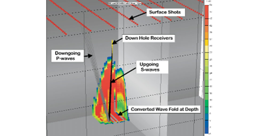
And depth? There are now an increasing number of cases where both sources and receivers have been placed in well bores. Phrases like “Cross well tomography” and “3D VSP” are becoming part of the exploration vocabulary. Figure 1 shows a typical 3D VSP situation, where the mode-converted wavefield, arising from surface sources, is recorded by downhole receivers. The design of geometries for such cases will carry different challenges than have been tackled so far.

And there are still problems to be solved on the surface:

• Building better 3D arrays.
• Canceling shot noise (linear and backscatter) with effective geometries.
• Multiples - is stack the best (the only effective?) weapon?
• Statics: How do geometries affect static calculations? - refraction and residual?
• Removing the effect of buried anomalies (dynamic statics) - what’s the best geometry?
• Determining velocities for 3D pre-stack time or depth? Can geometry help?
• 3D AVO? Is it possible to extract more formation information by designing 3D geometries specifically to enhance the response of various AVO parameters (offset range, reflection angle, etc.)?

Curse or not, these will be interesting times for all of us!