Abstract
This paper describes a new method of stratigraphic heterogeneity modeling in channelized reservoirs. A 3D model of a channelized reservoir is simulated by migrating and stacking multiple channels in a background facies, whereby reservoir flow units are represented based on geological rules rather than statistical distributions. Spatial distributions of major components of channel deposits, such as Inclined Heterolithic Stratification (IHS), abandoned channel infill, and overbank deposits, are represented in 3D based on their formation process and genetic relationships.
A synthetic seismic volume is generated from a channelized reservoir model in which locations and proportions of each facies are known. A workflow of seismic attribute generation and seismic facies classification procedure is applied to this synthetic seismic volume. Comparison of facies classification results from different attributes with a “ground-truth” geological model indicates a few pitfalls in seismic facies classification, especially with the selection of input attributes for classification. Facies strata-cubes derived from a voxel-based classification from multiple attributes is more consistent with the “ground-truth” geological model, whereas a 2D facies map obtained from trace-based seismic facies classification is not sufficient to reflect the spatial distributions of channelized reservoirs.
Introduction
Geological models are usually used in a qualitative manner in seismic interpretation. The objective of this paper is to illustrate that a quantitative representation of detailed geological models can provide insight into seismic attribute interpretation through facies classification. In the application of seismic attribute classification to mapping reservoir facies, one often faces such typical questions as:
- Which attributes should I use as input to classification?
- In the unsupervised classification method, how many classes should I use?
- In the hierarchical classification method, how many levels of hierarchy should I choose?
- Is the seismic facies corresponding to the geological facies? How could I cross-validate attribute derived facies models?
Whereas there are no unique and easy answers to the above questions, the objective of this work is to use seismic attribute classification results from a synthetic seismic volume generated from a 3D geological model that is regarded as “ground truth”. We consider a channelized reservoir for which seismic attribute analysis has proven to be very useful but results can be difficult to interpret.
The next section describes a 3D stratigraphic modeling approach for the channelized reservoir. The major channel components and parameterizations are illustrated with examples. This is followed by a summary of seismic attribute analysis and classification workflow applied to a synthetic seismic volume. Results of attribute classifications using a Self-Organized Map (SOM) (Kohonen 1989) and waveform correlation maps are compared in relation to different input attributes and classification parameters. The experiences learned from this synthetic example are summarized and the selection of attributes for facies classification are discussed.
3D Stratigraphic Models of Channelized Reservoirs
There are several computer-based methods to build 3D reservoir model flow simulations, such as the object-based method or cell-based geostatistical methods (Dubrule and Damsleth, 2001). However, none of these geostatistical methods is able to reproduce stratigraphic heterogeneity patterns at sub-seismic scale, which can be major controlling factors for fluid flow and spatial variations of acoustic properties. In this paper we report a newly developed modeling method to generate 3D stratigraphic architectures of channelized reservoirs. The modeling method is an extension of the bedding structure modeling method developed by Wen et. al (1998) and is being further developed in the SBED joint industrial project (JIP)1. The stratigraphic features within channelized reservoirs to be modeled in this study are below the resolution limit of conventional seismic data. The cell size is about 20 x 20 x 1 m3. At such a modeling scale, detailed geological features must be modelled based on their formation process, so that their 3D structures can be correctly represented in the geological model.
Models of single channel geometry
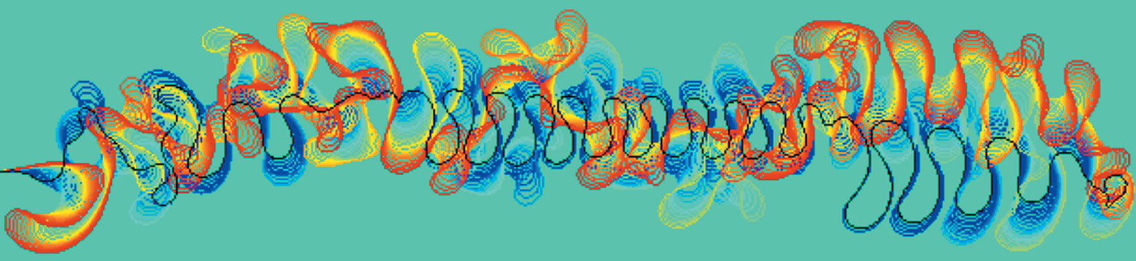
A channel’s 3D geometry at any given time in its development can be parameterized by its platform and section parameters. The channel platform location is represented by its central line, which can be a sine-wave or a simply a list of points that are digitized based on seismic data, a conceptual model, or simulated from other programs, such as the meandering channel central lines shown in Figure 1.
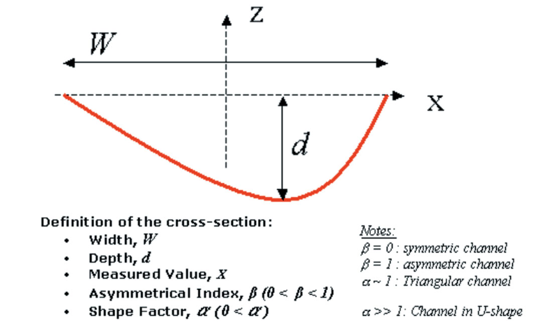
The section parameters (Figure 2) of a channel include: 1) maximum depth, 2) width, 3) asymmetrical index, and 4) shape factors. These four parameters normally vary along the central line. Such variation can be modelled based on deterministically derived rules –, such as one that says the steep side of the channel must be on the outer band – or rules specified by a trend –, such as making channel depth decrease or increase in a certain direction – or rules with a stochastic component, which are modelled by a one-dimensional Gaussian random function parameterized by a variogram model, mean and standard deviation. A surface representing the top of a channel system is constructed based on the channel-central line, its section parameters and the levee parameters describing the decay of elevation as a function of distance away from the channel central line (Figure 3).
Modeling components of channel deposits
What we regard as a channelized reservoir is formed by that channel’s deposition, migration and erosion processes during its “active” time. While these processes can be very complicated and involve both physical and chemical processes, we only modelled the geometrical aspects in our computer model. This is justified because our modeling objective is to reproduce a realistic 3-D stratigraphic framework at the sub-seismic scale. We modelled channel deposits into four components (Figure 4):
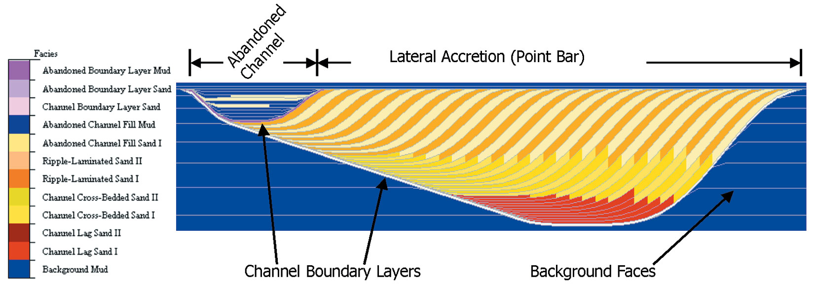
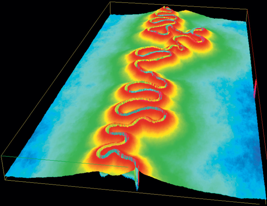
Lateral accretion: these are so-called point bar deposits formed by lateral channel migration. The lateral accretion is further modelled by four sub-components: channel lag deposits in the bottom, cross-bedded sandstone in the middle, ripple laminated sandstone on the top, and shale layers. Those lateral accretions that have shale layers are called IHS (Inclined Heterolithic Stratification). They are usually formed in tidal influenced channel systems; the McMurray formation in Alberta contains typical examples of this type of deposit. Figure 5 shows an example of lateral accretion simulated by SBED.
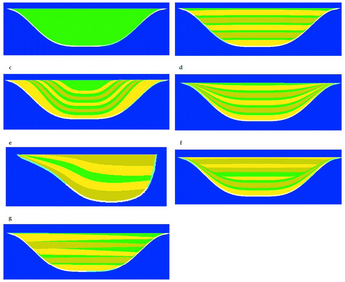
Abandoned channel fill: these are deposits filled into the last remaining spaces in the channel when it is abandoned (Figure 4). Depending on the geological setting, the abandoned channel fill pattern can be quite different. We have considered seven infill patterns as illustrated in Figure 6.
Overbank deposits: are regarded as background facies in our program. These include crevasse splays.
Channel boundary layers: To model the transmissibility between channel deposits and background facies or other channels, our channel model can include two types of boundary layers within channel deposits (Figure 4): a layer below all deposits of a channel and a layer below abandoned channel infill. If there is no lateral accretion component, only one layer is required to model the boundary. The reason to include a boundary layer as a separate modeling component is to explicitly represent model flow properties across one channel to another. Seismically, channel boundary layers could be a reflectors (assuming seismic resolution is good enough), since there tends to be a large contrast between sandy channel deposits and background mud facies.
Stacking Patterns of Multiple Channels
A channelized reservoir consists of deposits formed by multiple channels. Depending on base-level variation and tectonic setting, channel deposits are vertically stacked in different patterns. Whereas there are different geological terms to describe and classify channel stacking patterns, we model the stacking patterns based on channel amalgamation curves, which are typically used by geologists to describe the channelized deposits. Figure 7 illustrates the relationship between channel stacking patterns, channel intensity, and amalgamation curves.
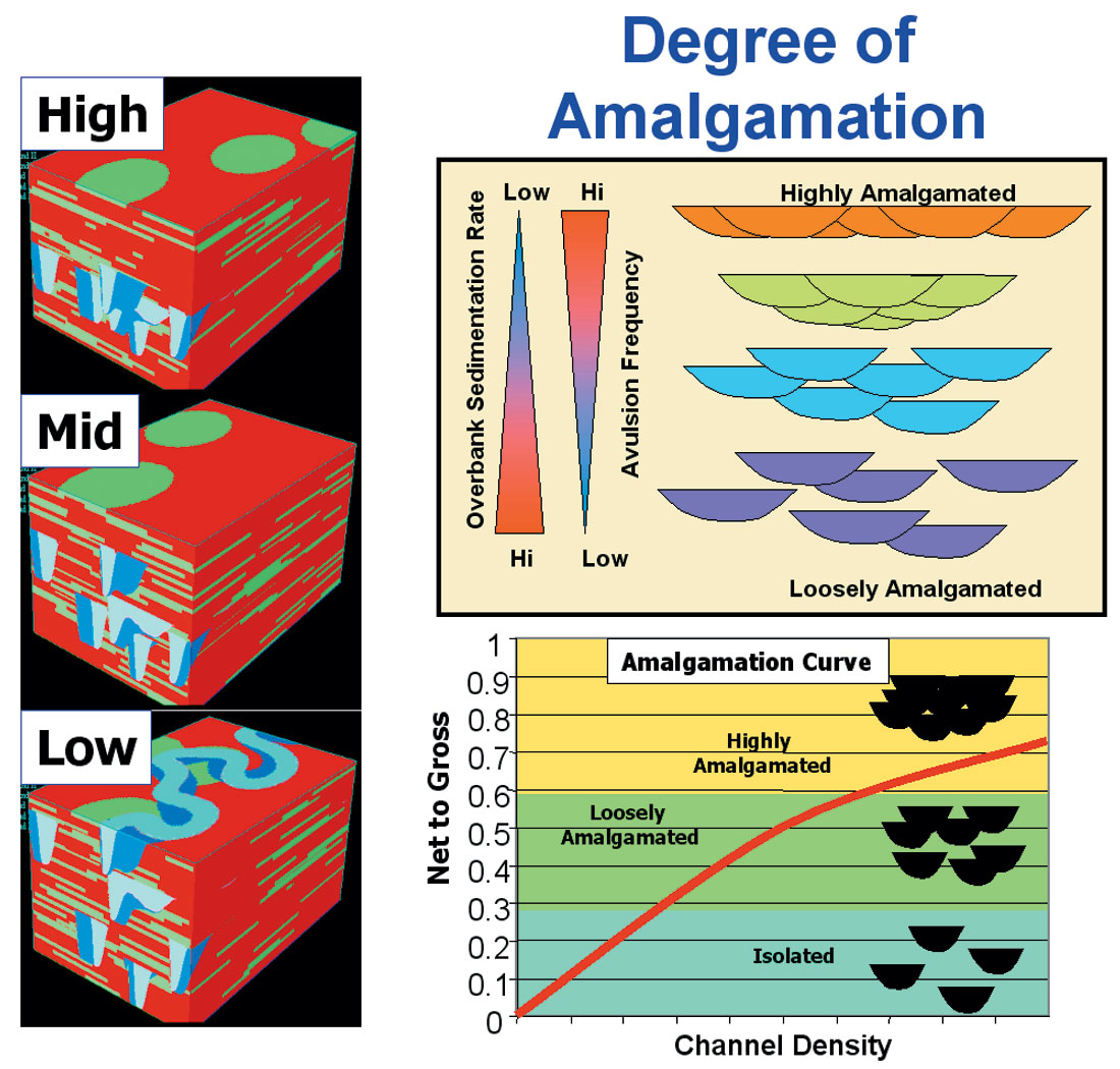
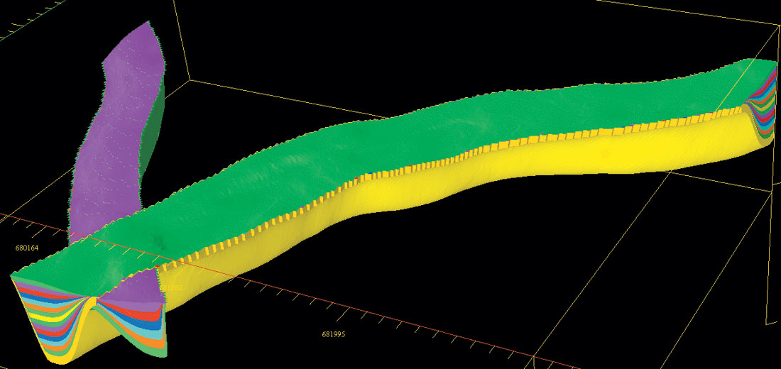
Figure 8 shows two channels with asymmetrical convergent infill patterns without displaying the overbank deposits. Channel migration, deposition and erosion in time-space domain leads to the formation of channelized reservoirs. Since bounding surfaces and internal stratigraphic variations are below the resolution of conventional seismic data, computer-based modeling based on knowledge of geological processes is the only way to reconstruct a realistic 3D model that captures detailed stratigraphic features.
Synthetic Seismic Volume and its Attributes
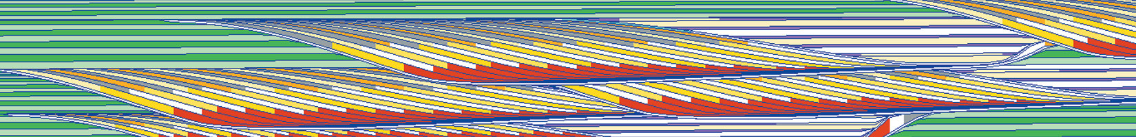
Figure 9 is a high-resolution (each sample is 20 x 20 x 1 m3) litho-facies model of a channelized reservoir. The model was simulated using the SBED program based on the principal described above. By assigning representative velocities and densities to each litho-facies, we then calculated an acoustic impedance cube, which was convolved with a Ricker wavelet with a peak frequency at 40 Hz. The resulting synthetic seismic volume is shown in Figure 9.
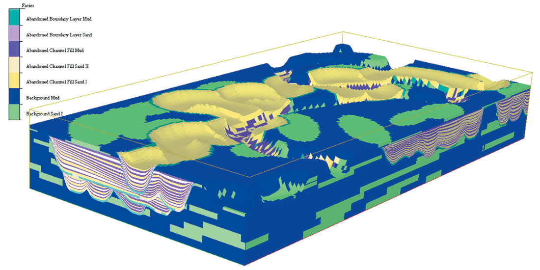
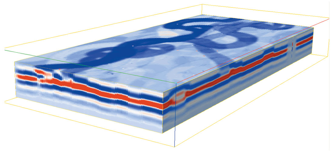
(b) synthetic seismic volume used in the attribute analysis and facies classifications (bottom).
Six post-stack attribute cubes were calculated from the synthetic seismic volumes. They are instantaneous amplitude, weighted instantaneous frequency, instantaneous phase, relative acoustic impedance and semblance. These attributes are easy to calculate. We did not consider any pre-stack attributes in the following comparison study. It is just a matter of CPU time to compute more attributes. The major challenge in the application of seismic attributes to reservoir mapping is how we interpret the multiple attributes, i.e. link what we see on seismic attributes to reservoir properties, such as lithology, and hopefully fluid content.
Seismic facies classification
Seismic facies classification is a computation process to assign each trace in an interval or each sample to a facies code. Depending whether training data are used in the classification procedure, there are supervised and unsupervised classification methods. In this study we considered an unsupervised classification method based on the Self-Organized Map (SOM) (Kohonen 1989) method, which is preferred over more the traditional clustering method (Thiery, et al., 2003). Since we know the “ground-truth” of the seismic volume in the synthetic data (Figure 9), we should be able to identify which attributes are more effective than others when they are used as input to the classifier.
Depending on whether classification algorithms are applied to a trace in an interval or each sample (a voxel) in the seismic volume, the seismic facies classification can be trace-based or voxel-based. We examined both trace-based and voxel-based SOM methods applied to the six attributes calculated for the synthetic seismic volumes.
Strata-Cube
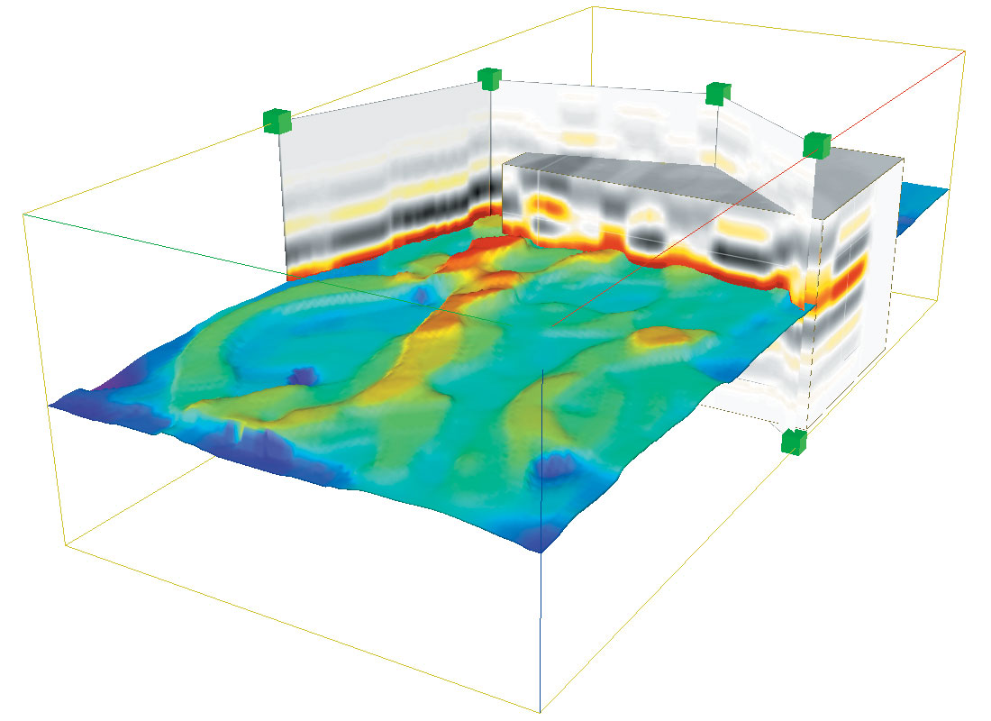
The first step is our seismic classification method is to define a stratigraphic volume, which we call a strata-cube. A strata-cube is a sub-volume bounded by two horizons, which are not necessarily parallel. Figure 10 show the seismic horizon tracked from the synthetic seismic volume. It is a strong reflector in the middle of the channelized reservoir. A strata-cube with a constant thickness of 20 milli seconds was defined around this horizon. We then applied to both trace-based and voxel-based SOM classification methods to the data set.
Trace-based seismic facies classification
In a trace-based seismic facies classification, we assign one facies code to each trace within a strata-cube; hence vertical variations of facies within the interval would be unmappable. This may be acceptable in consideration of the seismic resolution limit compared with the scale of vertical facies change. But in areas where vertical changes in facies are detected (not necessarily resolved) by the attributes, a facies map from tracebased classification would not be sufficient.
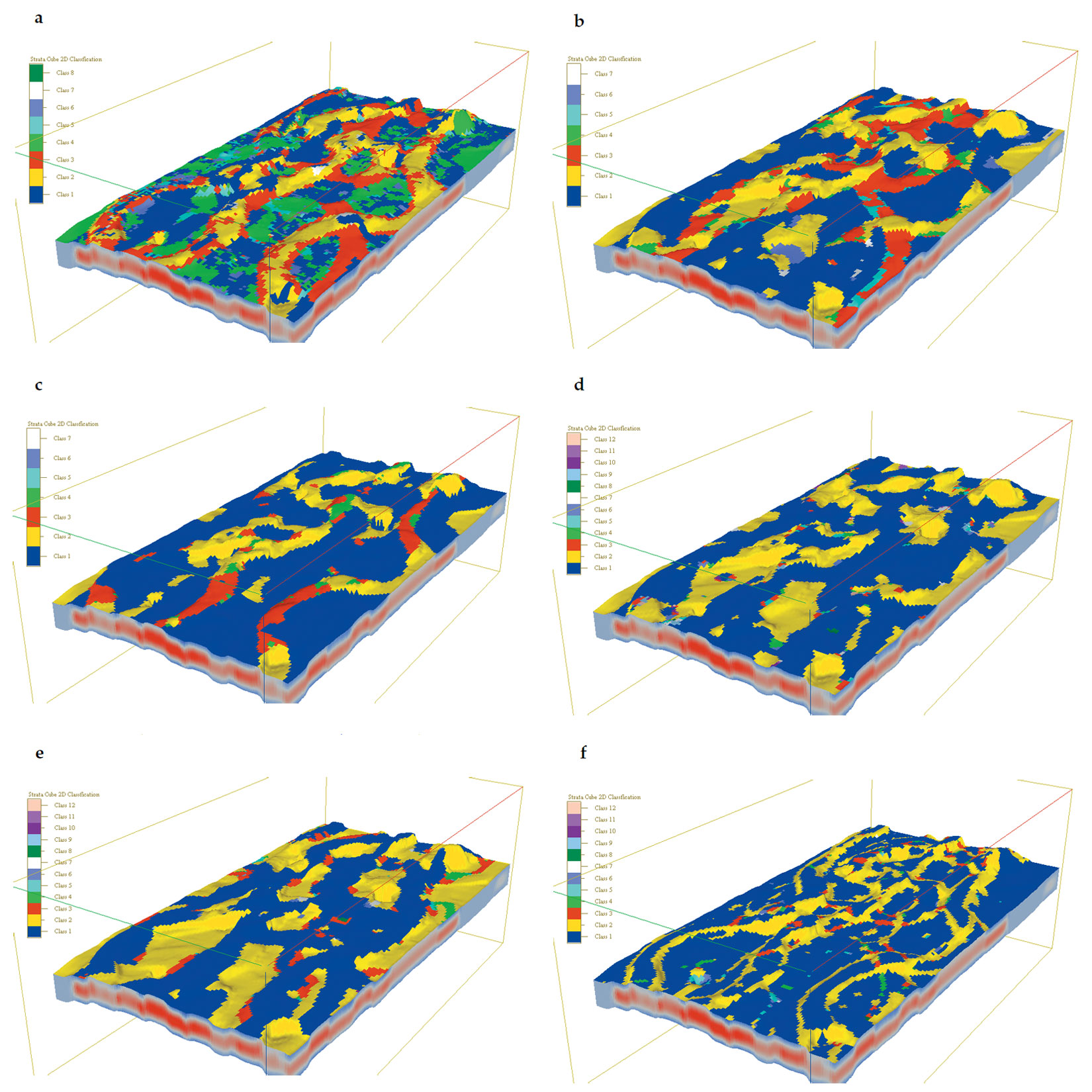
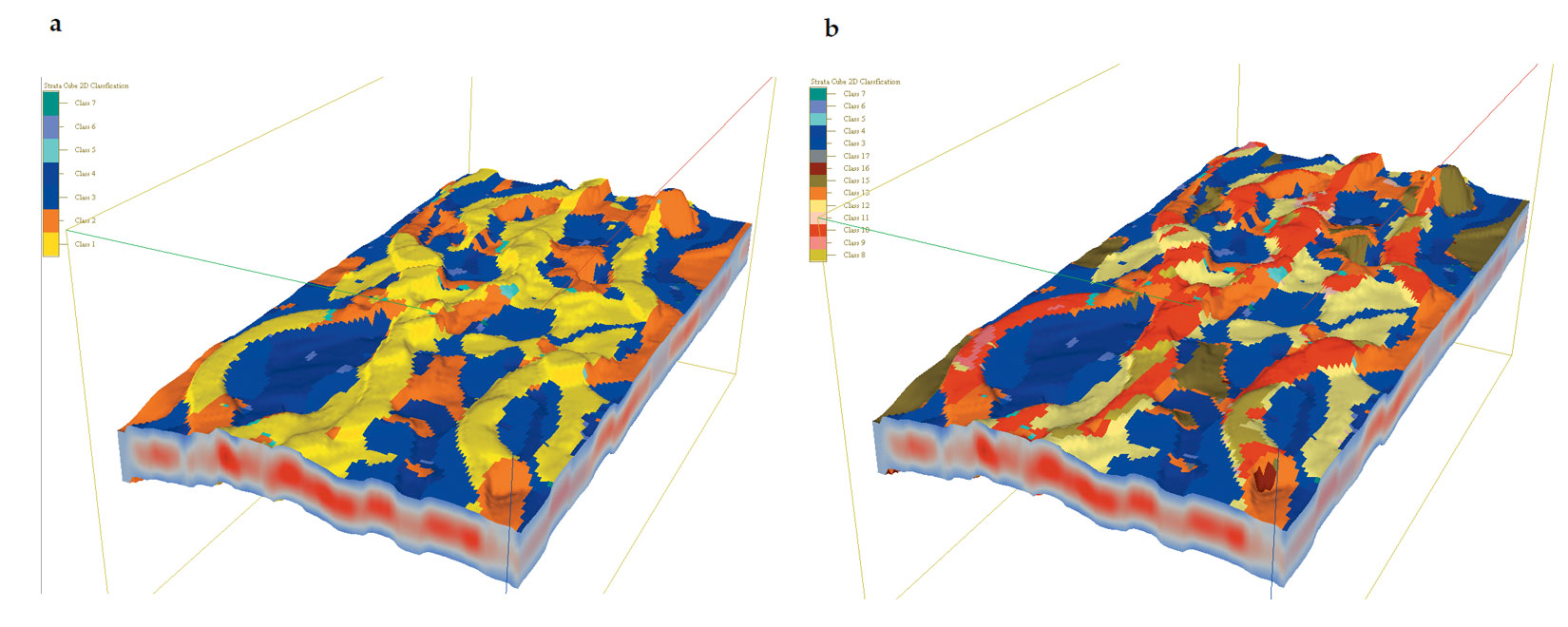
Figure 11 displays six seismic facies maps are wrapped on the top-surface of the strata-cube. Only one attribute is used in each classification in order to examine the effectiveness of individual attributes. Whereas a 2D facies map is not sufficient to represent the 3D heterogeneity of facies variation below the seismic resolution, it nevertheless reflects a general trend on a map view. It can be observed that facies maps classified from average weighted frequency and instantaneous amplitude are the best among the six attributes. Facies from instantaneous phase is sensitive to interval definition. It is not surprising that the facies map from the semblance attribute reflects more boundary information of channels that the litho-facies information.
Our method of trace-based classification can utilize multiple seismic attributes within a strata-cube. Since single attribute facies maps from average weighted frequency and instantaneous amplitude looks more meaningful, we then use both these attributes in a multi-attribute trace-based classification. The resulting facies map is shown in Figure 12. The seismic facies pattern looks more consistent with our “ground-truth” geological model Figure 9. However, the internal variations within channel infill deposits are not reflected in Figure 12. An interactive hierarchy classification scheme is then selectively applied to facies 1 and 2, which corresponds to channel-infill facies. The result is shown in Figure 12. It can be seen that the hierarchy classification scheme can be an effective approach to mapping internal facies variation, given that the top-level facies map is properly derived.
Voxel-based seismic facies classification
In the voxel-based seismic facies classification, each sample (a voxel) is assigned a facies code based on one or multiple attributes at the sample. Results from voxel-based classifications are facies volumes. Given that a seismic data set has enough resolution, voxel-based facies classification would be able to map vertical facies variation within a reservoir.
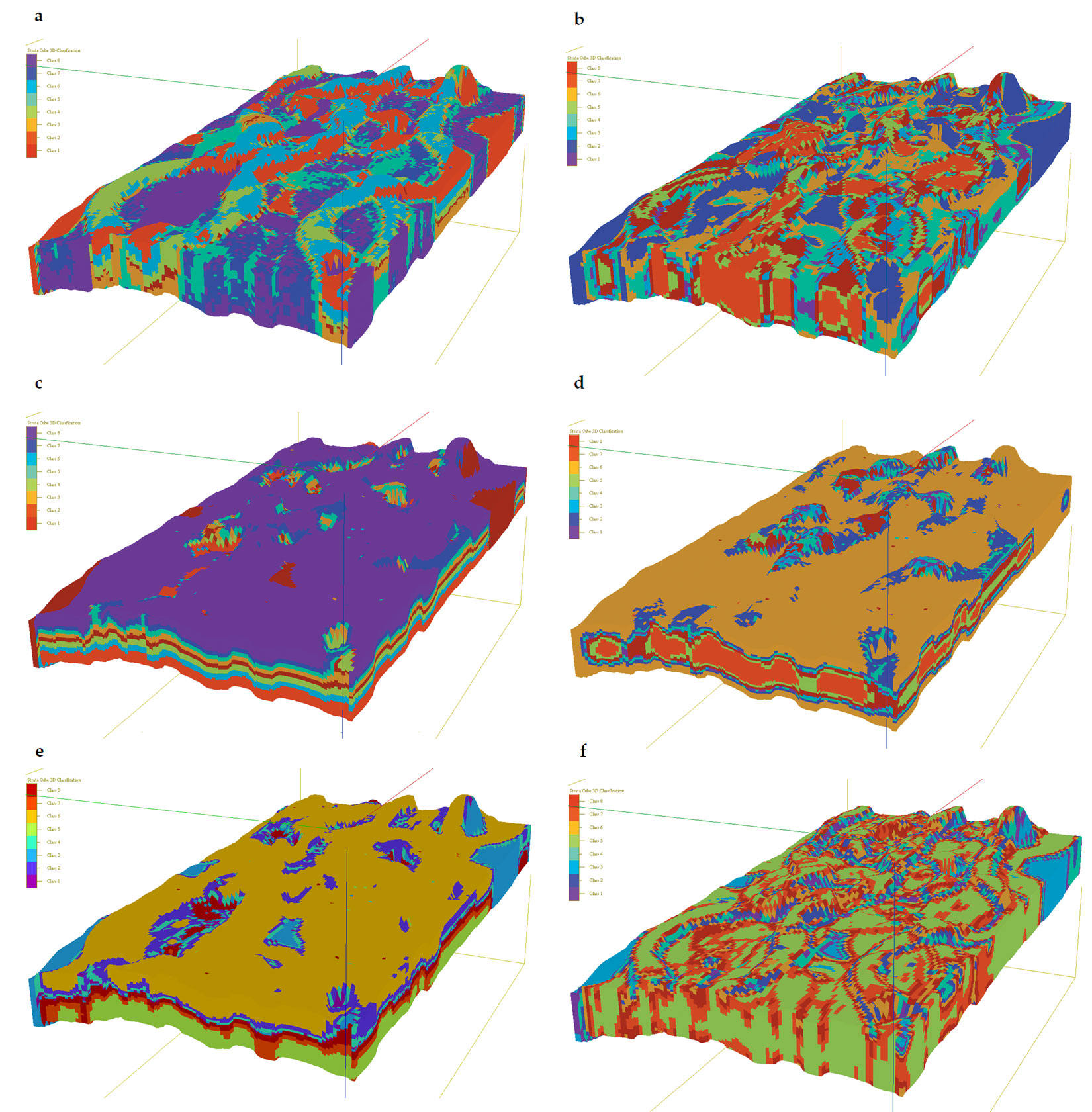
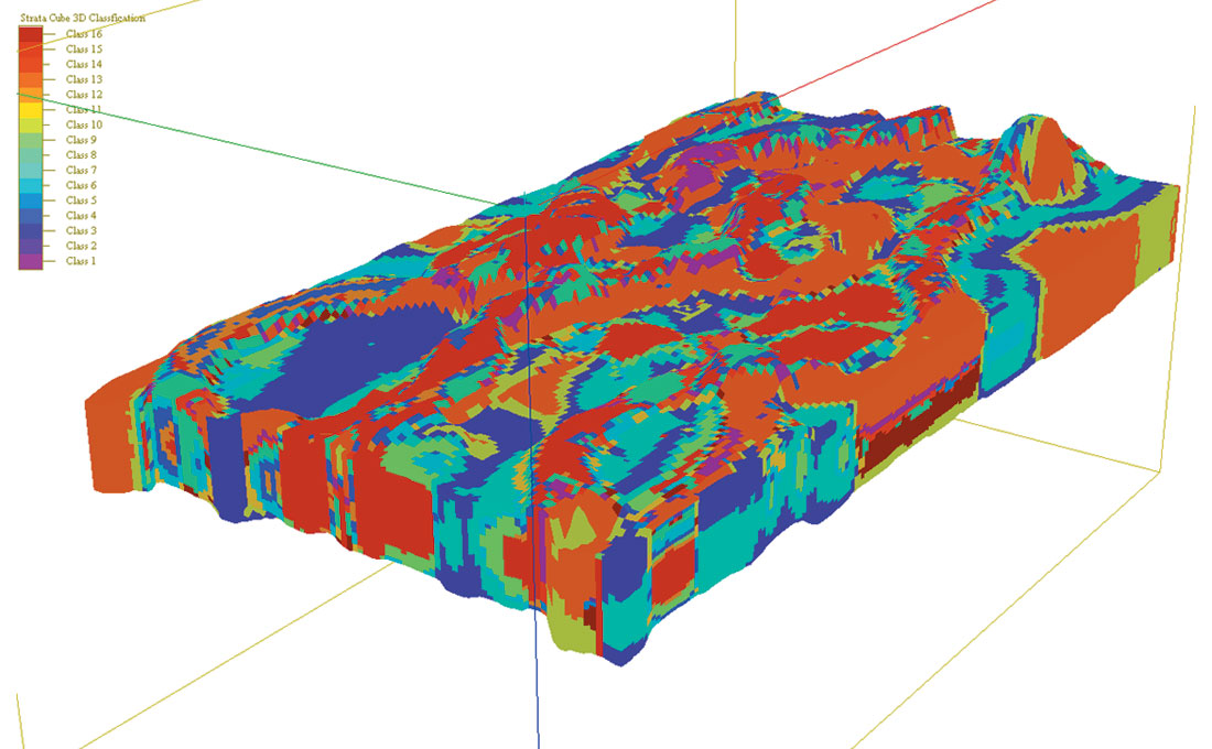
In the same procedure as the trace-based classification, we first use each of six individual attributes to derive a seismic facies volume (Figure 13). The result is consistent with what we observed from the trace-based classification map (Figure 11). Only using average weighted frequency and instantaneous amplitude can result in a facies pattern comparable to the “ground-truth” litho-facies cube (Figure 9). We find using more attributes in a seismic facies classification does not necessarily improve the classification results, if some of the input attributes have no direct link to what is to be classified. But combining multiple attributes that are related to the reservoir properties we want to map (in this case it is the litho-facies that we want to map), will generally improve the results (Figure 14).
Summary
In this paper we presented a geological modeling method to generate detailed 3D stratigraphic architectures of channelized reservoirs. Using this detailed model as the “ground-truth”, we created a synthetic seismic volume to which the attribute analysis and seismic facies classification were applied. Both trace-based and voxel-based seismic facies classification procedures were applied to the synthetic data. By comparing the seismic facies classification results with the “ground-truth” litho-facies model, we observed that average weighted frequency and instantaneous amplitude are more effective than other attributes considered in this study as input to the seismic facies classification for mapping litho-facies.

Acknowledgements
We thank the support of SBED JIP member companies for the development of SBED products, which make it possible to carry out the work reported in this paper. Any opinions expressed in this publication are those of the author and do not necessarily reflect the views of SBED JIP member companies.


Join the Conversation
Interested in starting, or contributing to a conversation about an article or issue of the RECORDER? Join our CSEG LinkedIn Group.
Share This Article