2D and 3D Anisotropic Depth Migration Case Histories

Abstract

Anisotropic depth migration (ADM) has become more commonplace over the past four years. The data-processing examples detailed here illustrate the robustness of the method in a variety of structured settings in the Alberta Foothills. The public-domain structural line, the Husky/Talisman dataset, illustrates subtle improvements in imaging with a dramatic improvement in accuracy of horizon depths when ADM is applied to these data. A3D survey in a difficult imaging area, Nordegg/Chungo, shows significant healing of broken basement reflectors when we correct for anisotropy in the complex-dipping clastic overburden. Finally, in the Blackstone area where we observe intense folding in the near surface, comparisons between poststack time migration, prestack time migration, prestack depth migration, and prestack anisotropic depth migration in the Blackstone area show the similar step-change improvements as we improve the technology of our algorithm.

Introduction

Traditional depth migration corrects only for lateral velocity heterogeneity. Current anisotropic depth migration algorithms also correct for velocity changing with direction in the dipping clastic overburden. Seismic anisotropy is a well-quantified physical characteristic of clastic rocks. Studies of anisotropic behaviour in clastic rocks include Thomsen (1986), Vernik and Liu (1997), Leslie et al (1997). Several papers over the past seven years illustrate the improvements in imaging when we stop ignoring anisotropy and begin to correct for it (Ball, 1995; Vestrum and Muenzer, 1997; Vestrum, et al., 1998; Ferguson and Margrave, 1998; Schmid et al., 1998; Dai et al., 1998; Fei et al., 1998; Vestrum et al., 1999, Kirtland Grech et al, 2001; etc.).

The seismic data processing case histories presented here outline the improvements in seismic imaging and structural positioning when we correct for seismic anisotropy in depth migration.

Benjamin Creek

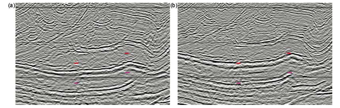
The Husky/Talisman dataset is the focus of our first processing case history. In this example, I illustrate the improvement in correlation between well depths and seismic depths. Figure 1 shows this improvement. Isotropic depth migration for this line (Figure 1a) shows a typical result (Shultz and Canales, 1997; Etris et al., 2001) of isotropic depth migration where the seismic depths are deeper than the well depths. When we ignore anisotropy, we need to use a velocity faster than the vertical velocity if we are to flatten the image gathers and obtain a quality image. The anisotropic migration (Figure 1b), models the velocity behaviour changing with direction, so it produces a clear image and correlates to the well depths. One can see in Figure 1b that there is still some uncertainty in the correlation, but we have removed a systematic error from the depth correlation. We could now go back and adjust our imaging velocities so that our final depth migration matched perfectly with well depths, without needing a separate depth-conversion step after the depth migration. We can now consider well depths as a constraint on our imaging velocity model. There are also several imaging improvements on the anisotropic depth migration over the isotropic depth migration.

Nordegg/Chungo

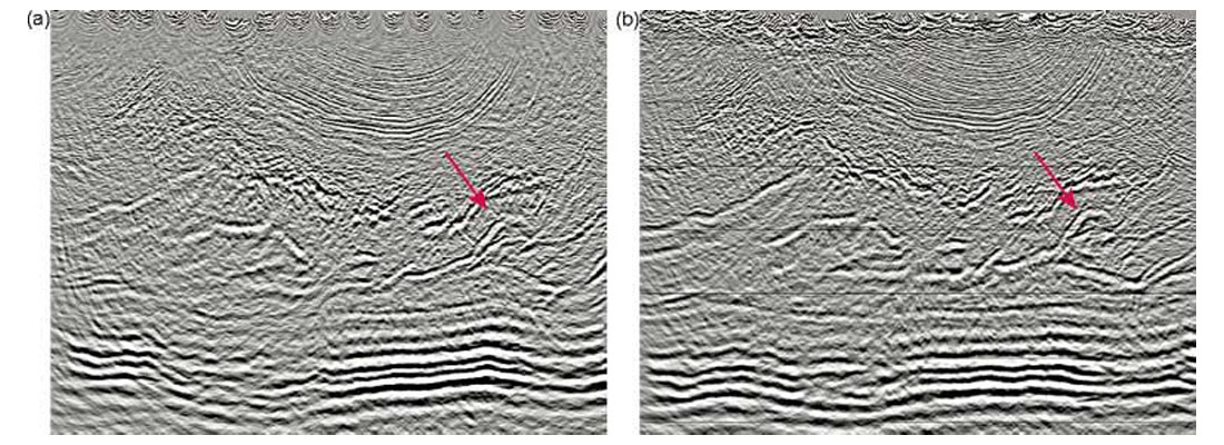
The Nordegg/Chungo 3D is a Time Seismic data volume acquired in the Alberta Foothills. A more difficult imaging area than the Benjamin Creek area, this volume shows imaging problems that arise when the anisotropic overburden has dramatically changing dip. Figure 2 shows the comparison between isotropic and anisotropic depth migrations for a line out of this volume. Note the improvement in basement continuity beneath the steeply dipping near-surface when we use anisotropic depth migration (Figure 2b). Several other potential hydrocarbon-target events show similar improvement. Note that the target event, as indicated by the red arrow, shows more consistent imaging over the range of dips from the back limb over the crest of the structure and into the forelimb. The anisotropic velocity model more accurately represents the velocity structure of the overburden. With more accurate raytracing over a larger range of reflector angles, the migration is better able to image the range of reflector dips on this structure.

Blackstone

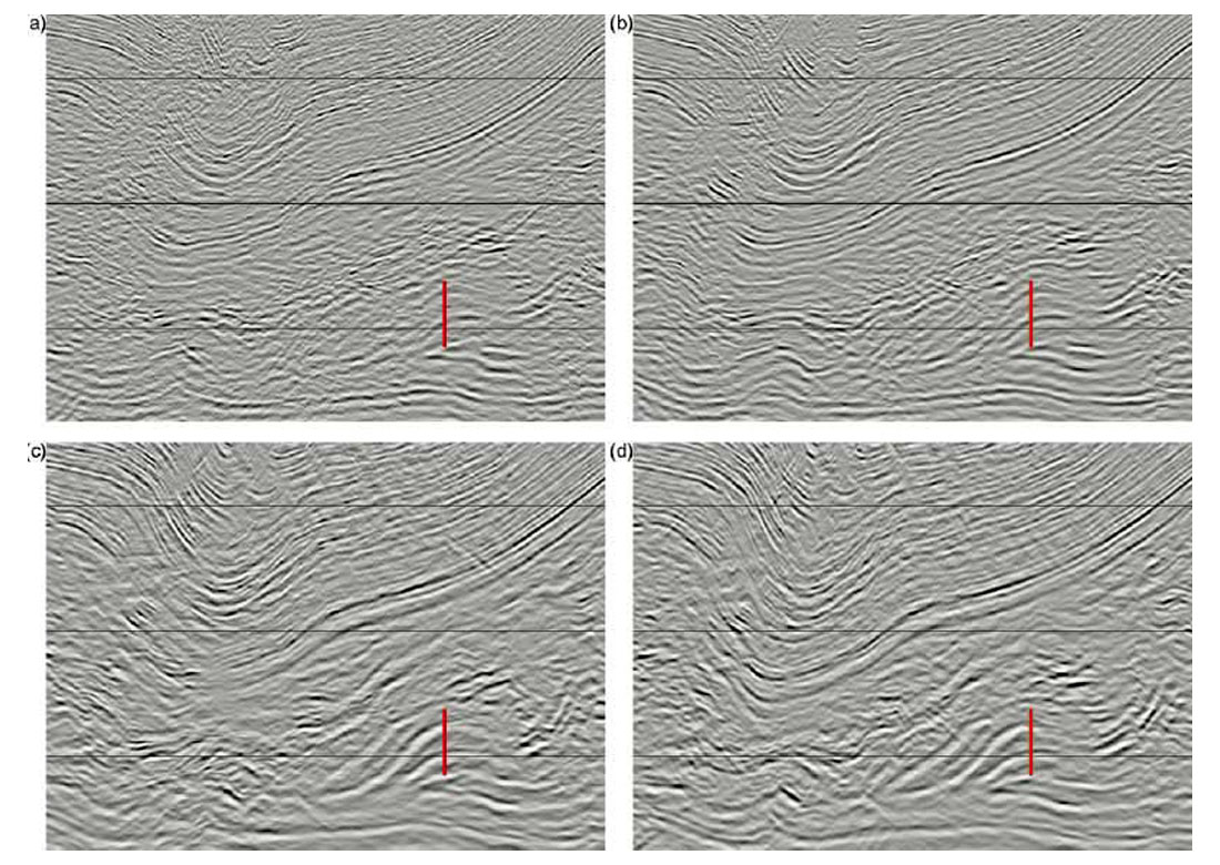
This Talisman dataset is a very dramatic anisotropic imaging example. The extensive folding of the clastic overburden creates difficulties imaging structures below. Figure 3 shows a comparison between poststack time migration (Figure 3a), prestack time migration (Figure 3a), prestack depth migration (Figure 3c), and prestack anisotropic depth migration (Figure 3d). Each step forward in complexity of the migration has its own step improvement in imaging. The red marker is plotted at the same position on each of the four seismic displays in Figure 3 to show the lateral position change of the target events between the four migrations. A more dramatic difference between these migrations, however, may be the imaging of these target events. In the poststack-time migated (Figure 3a) section, we see one target structure. The prestack-time migrated section (Figure 3b) images the target event more clearly and images a possible second sheet above the main target. This second sheet is bright and continuous after prestack depth migration (Figure 3c), and the depth-migrated section also shows a possible third sheet to the left of the second sheet. This third sheet is more clearly defined after anisotropic depth migration (Figure 3d) and all of the target events show sharper truncations. Further discussion of the processing technologies applied to this particular dataset, please refer to Gray et al. (2002).

Conclusions

Anisotropic depth migration reduces the overall depth error on a depth migrated section by removing a systematic anisotropy error from our data. We can then use the well depths to calibrate our anisotropic velocity model to simultaneously optimize image quality and depth accuracy.

As we increase the complexity of our velocity modelling, our migration can images sharper reflector terminations and a larger range of reflector angles. In the data example shown here, the imaging improvements of anisotropic depth migration over isotropic depth migration are comparable to the imaging improvements of depth migration over time migration and prestack time migration over poststack time migration.