2-D Migration Footprint

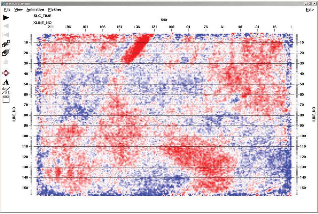
It is sometimes thought that prestack migration footprint is a 3-D problem that is due to the poor spatial sampling inherent in prestack 3-D data. Footprint is often visible on 3-D time slices as a hatched interference pattern, as in Figure 1. However, it is not always recognized that prestack migration can generate a characteristic footprint on 2-D data as well as 3-D data. It is worthwhile to work through a simple example of how footprint is generated on 2-D data so that the 3-D problem becomes more understandable.

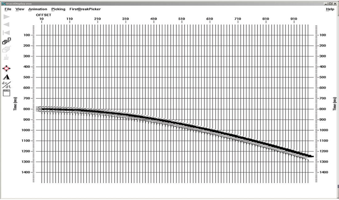
A decimation test with an extremely simple model is sufficient to show how footprint is generated by 2-D prestack time migration once the source interval exceeds the receiver interval. We put a single flat reflector at 400 m depth in a constant velocity medium of 1000 m/s. The receiver interval is 10 m, and the full dataset (before decimation) has a source interval of 10 m. We generate 61 end-on shots, each with 96 channels, using a Kirchhoff modelling algorithm. Figure 2 shows one of the unmigrated shot gathers. The synthetic seismograms have been generated with a 30 Hz Ricker wavelet.

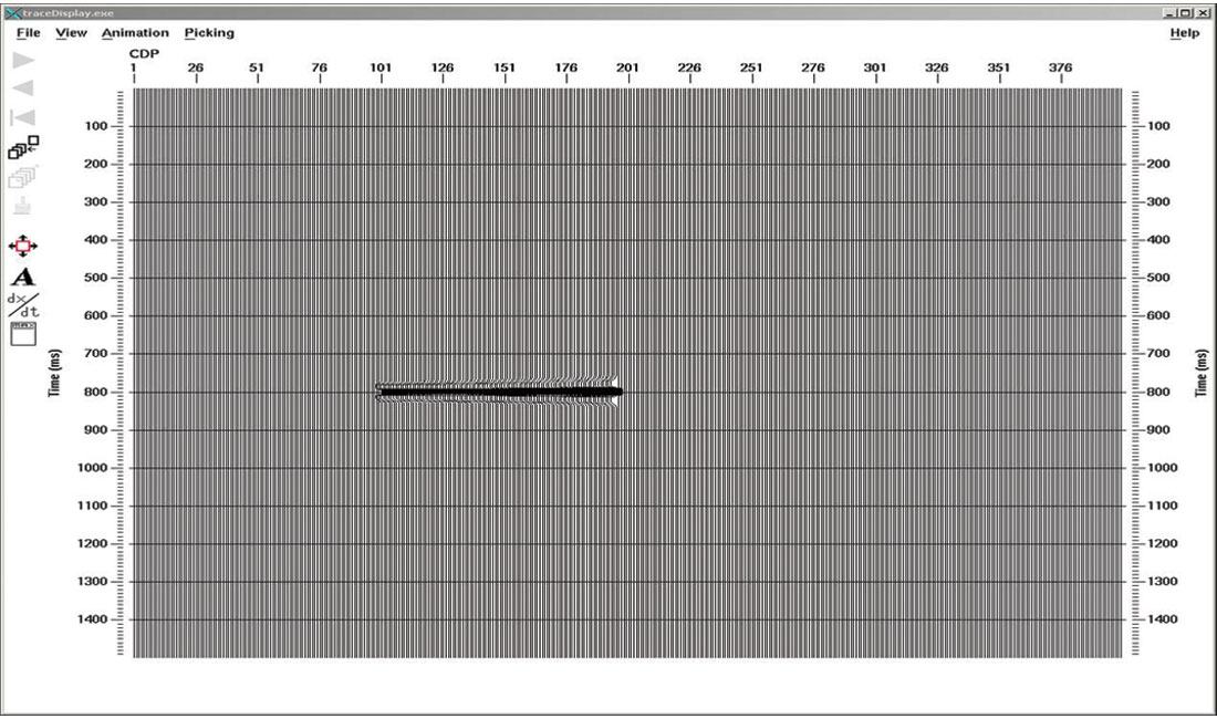
The advantage of using such a simple model is that it is very simple to generate the correct migrated image. In fact, NMO-stack produces exactly the right result for a flat reflector, so we will be most happy if prestack migration of each shot gather could produce as good a result as the NMO-corrected source gather in Figure 3. Notice that NMO-stretch reduces the resolution of the reflector on the right-hand side. If we prestack migrate the same source gather with a Kirchhoff algorithm, we get the result in Figure 4. Notice that the flat reflector is positioned correctly, along with the NMO-stretch, but there are prominent migration smiles that look as though they have been generated by the left and right ends of the shot gather.

One way of understanding how these migration artifacts have been generated is by taking a quick look at how the integrals in Kirchhoff migration are evaluated. The migration of each source gather is given by an integral of the form:

We are obviously not worrying about the exact details of the integral here. The factors within the square brackets […], if they were included, would include functions that determine exactly how the weighted summation of the shot gather at location xs along hyperbolic trajectories is done across the input shot gather p(t, xs, xr), as a function of time, t, and receiver position, xr.

Although the integral over receiver position has limits from minus infinity to plus infinity, we only have receivers that extend from the beginning to the end of the receiver spread. Therefore we truncate the integral at the beginning and end of the receivers by ignoring the first and third terms in this equation:

The origin of the artifacts in the migrated image of Figure 4 is due to the fact that we are only evaluating the middle term in this equation, and ignoring the other two.

The prestack migration algorithm includes an integral over sources, as well as receivers:

In general, the integral over shots is simply converted into a summation, regardless of the number of sources, or the interval between source locations. Once again we must truncate an integral because we only have sources from the beginning to the end of the seismic line:

We evaluate only the middle term in this equation and neglect the first and third term, which is what generates the familiar edge effects at the beginning and end of the seismic line that we encounter even with poststack migration.

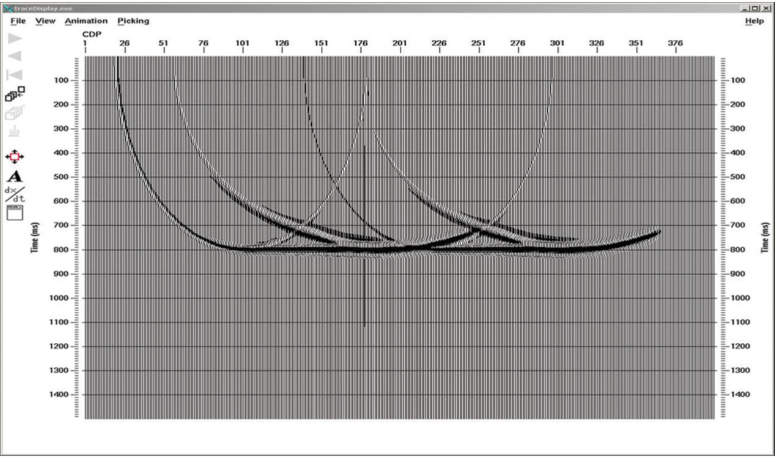
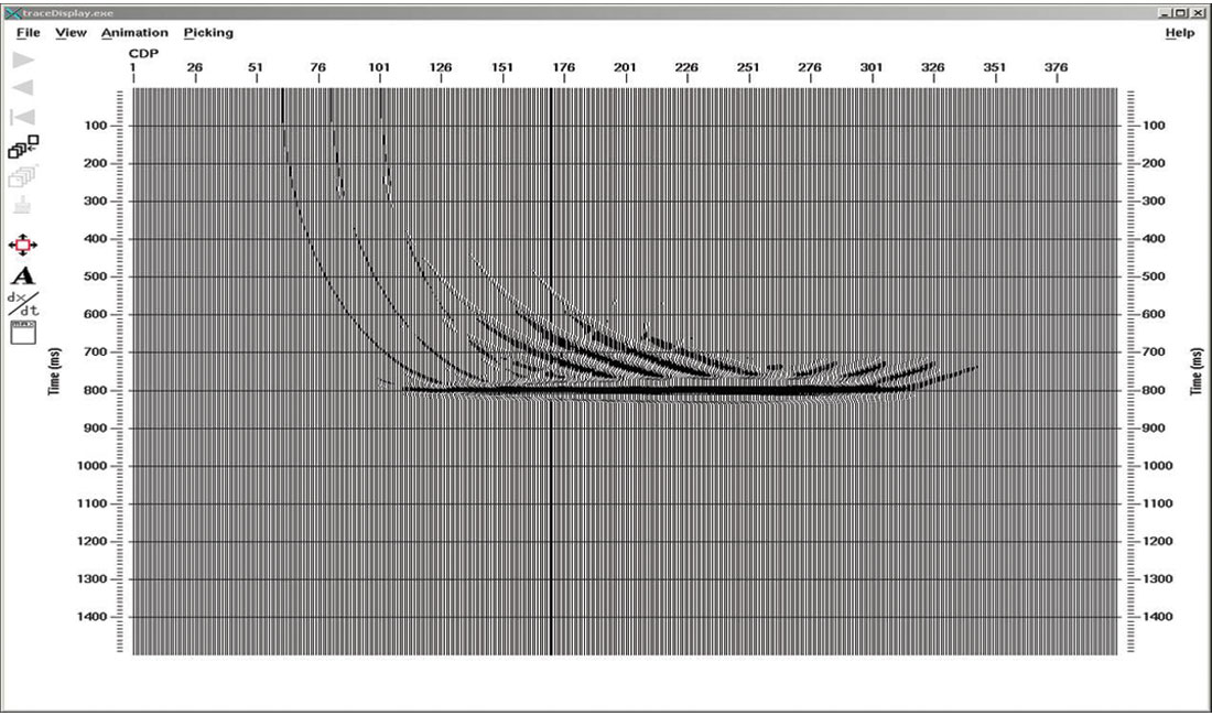
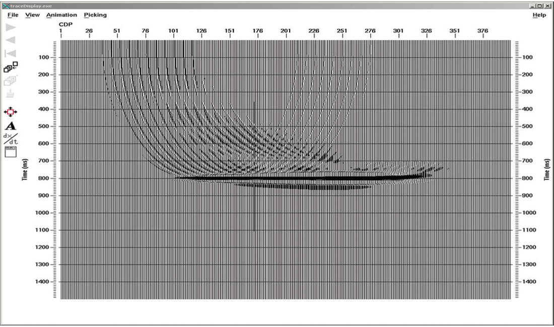
Figure 5 shows the image with two migrated shots. The flat reflector is relatively well imaged, but the edge effects from each shot are obviously not cancelling each other out at all. Figure 6 shows the results with 6 shots (shot interval = 10 x receiver interval). The pattern of edge effects now looks quite regular, like something we would call a footprint. What shot interval needs to be used for the edge effect from one shot to merge smoothly with the edge effect from the next shot, so that the edges disappear?

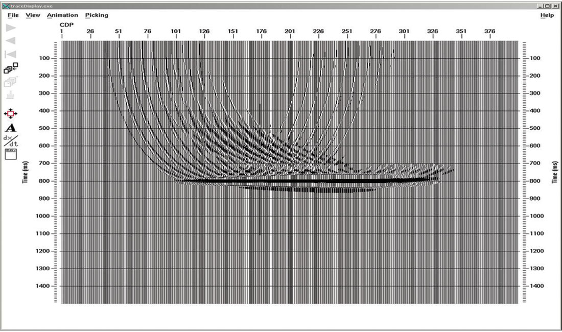
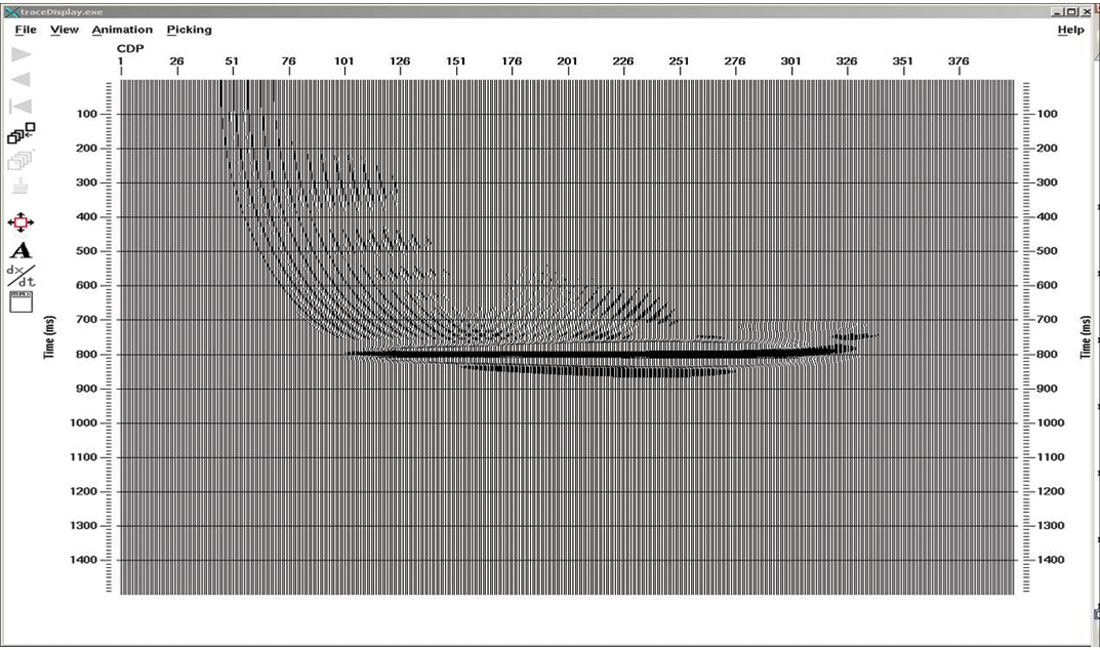
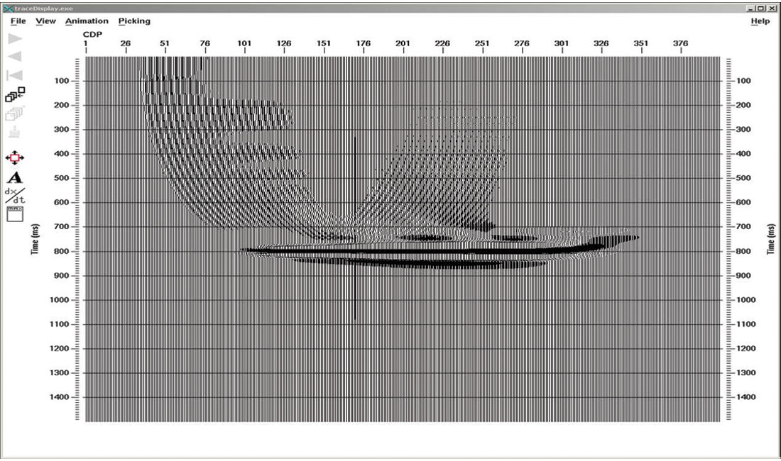
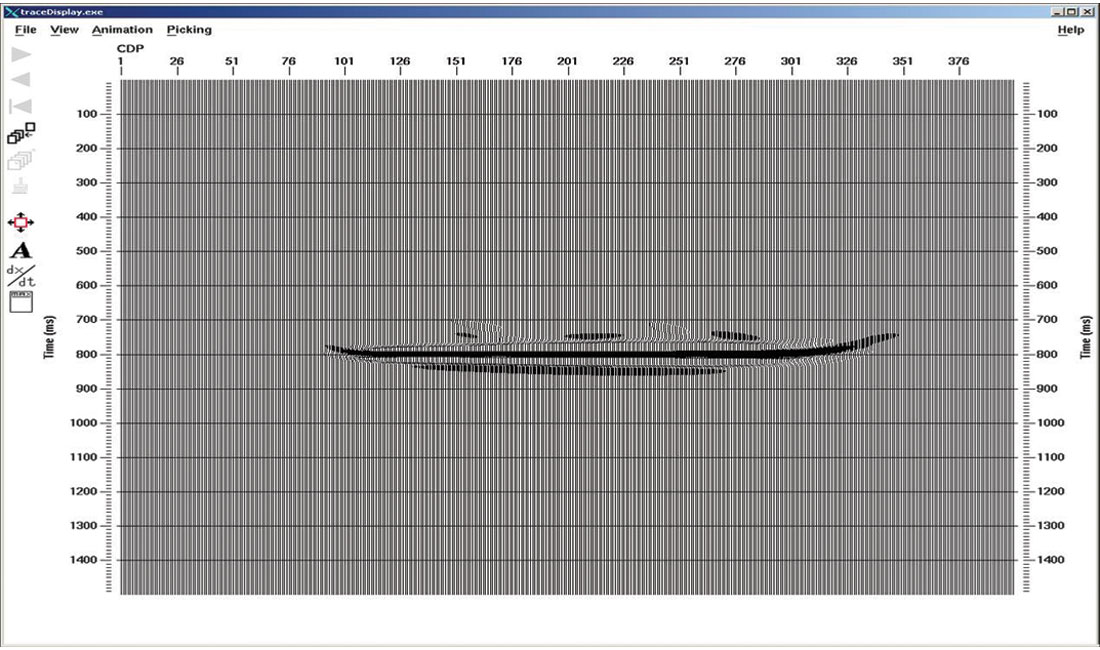
Figures 7 to 11 show the migrated images as the shot interval is reduced from 5 times the receiver interval to a shot interval that is equal to the receiver interval. The interference pattern of edge effects (the migration footprint) does not fully disappear until the shot interval equals the receiver interval. Figure 12 shows the image from the NMO stack of all 61 shot gathers. The best prestack migrated result (Fig. 11) is not quite a good as the NMO stack because it has edge artifacts at the beginning and end of the seismic line.

The purpose of this short article is to illustrate that migration footprint is a problem with 2-D data as well as with 3-D data. The simple example used in this article has also shown that, without any additional compensation, migration footprint arises in 2-D prestack migration once the shot interval is greater than the receiver interval.