Characterization of a heavy oil reservoir combining multiattribute analysis and spectral decomposition for density prediction, Maturín Sub-basin, Venezuela

Summary

The main objective of this work is to characterize a heavy oil reservoir located at the southern flank of the Maturín Sub- Basin. A rock physics analysis showed that the acoustic impedances of sandstones and shales are very similar within the reservoir, but density is a good lithological indicator. Hence, a multiattribute analysis for density prediction seemed to be the best choice for mapping the reservoir sandstones. We tested linear and nonlinear (Probabilistic Neural Network (PNN) and Multi-Layer Neural Network (MLFN)) multiattribute transforms, between a subset of attributes and density log values. The best results, measured in terms of cross-validations, were obtained using the MLFN transform. This transform was applied to the entire seismic data to generate the pseudo-density volume.

A model-based acoustic inversion was also performed to include the acoustic impedance volume as input in the multiattribute analysis. However, we were unable to observe anomalies associated with the reservoir sandstones in the Pimpedance volume possibly due to the acoustic impedances behavior within the reservoir. Since the reservoir is characterized by the presence of channels and bars (López and Aldana, 2007), we decided to perform a spectral decomposition analysis of the seismic data trying to map the geobodies. This decomposition allowed a good identification of stratigraphic features and the frequency volumes were included in the multiattribute analysis. The density prediction was improved using spectral attributes and, therefore, a better delineation and reservoir characterization was accomplished.

Introduction

In general, estimation of petrophysical properties using only acoustic impedance generated from poststack 3D data volume may not be reliable. This is due to the inherent characteristics of seismic data (i.e., its band-limited nature, amplitude- scaling effects and the presence of noise). It is also related to the non-uniqueness nature of the inversion schemes due to their dependence on the initial models (Pramanik et al., 2004). Different geostatistical techniques have been used trying to estimate petrophysical properties out from seismic data, tied to well information (e.g. Russell et al., 2001; Pramanik et al., 2004). Attributes derived from multiattribute analysis of seismic data to predict log properties have been used to obtain 3D pseudo-properties volumes that help in the characterization of different reservoirs. Some of these approaches use multilinear stepwise regression and neural networks (Hampson et al., 2001). In all these cases, the statistical methods are used to find a relationship between the attributes and well-log data, as well as obtaining a multiattribute transform that gives the best fit between seismic and well log information at the tie points (i.e. well locations). This fit is evaluated via cross validation tests.

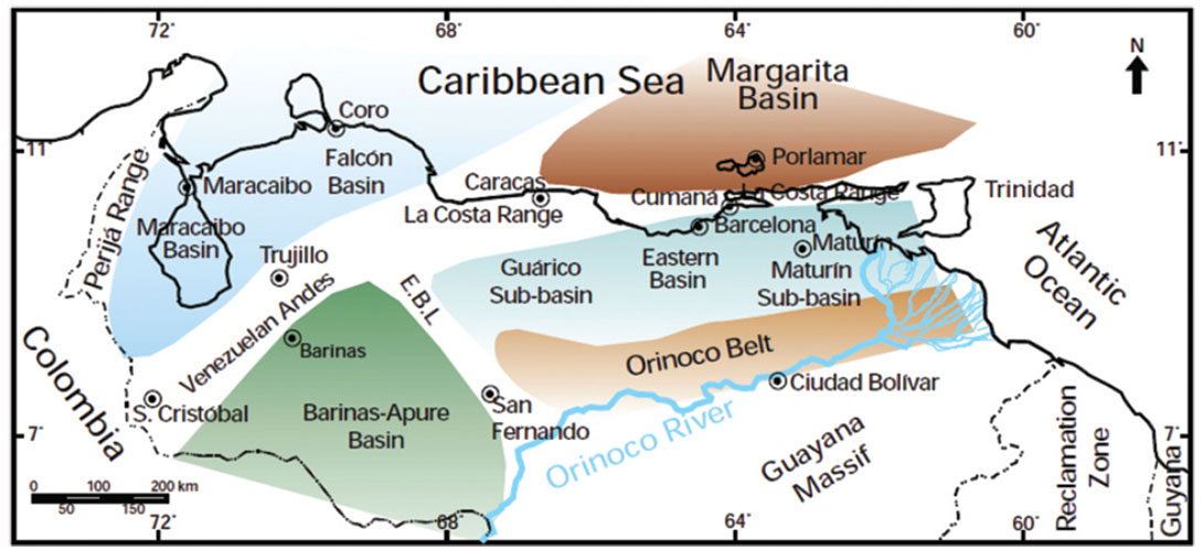
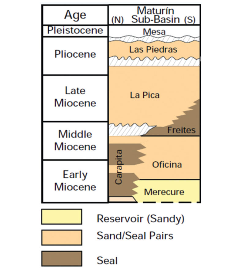
Following this approach, in the present work we attempt to go beyond the conventional seismic inversion by predicting log properties, other than acoustic impedance, using seismic attributes (e.g. Hampson et al., 2001 and Cedillo et al., 2004) in a heavy oil field. The derived relationship between seismic attributes and log values is statistical rather than deterministic. We study Early and Middle Miocene reservoirs, located at the southern flank of the Maturín Sub-Basin (Eastern Venezuela Basin) (Figure 1). The producer unit corresponds to interbedded heavy oil-saturated sandstones and shales from the basal part of the Oficina Formation (Figure 2). These reservoirs are mainly composed of sandstones of deltaic to shallow-marine environments with a stratigraphic evolution that ranges from thick channels to shaly interdistributary zones (López and Aldana, 2007). The complex geological setup of these heavy oil fields leads to both, lateral and vertical heterogeneities that are found difficult to capture by performing only conventional poststack seismic inversion (Cuesta et al., 2009). In addition, the acoustic impedances of sandstones and shales within the reservoir are found to be very similar. This fact bolsters the application of techniques such as multivariate analysis and Neural Networks in order to derive a volume of a pseudo-property that leads to an effective characterization that seismic inversion alone may not be effective in doing. The relationship will be obtained using 11 training wells and 1 validation well. The transform with the highest cross-correlation at the validation well, will be applied to the entire seismic volume, which comprises an area of 90Km2. Frequency, phase, filtered-seismic data, derivative and integrated attributes, and an acoustic impedance volume will be used in the multiattribute analysis. Another input for deriving the multiattribute transform are the frequency volumes obtained from the spectral decomposition analysis of the seismic data.

Rock physics and acoustic inversion

A rock physics analysis, based on crossplots of different petrophysical properties, was first performed to understand and discriminate the reservoir lithological properties.

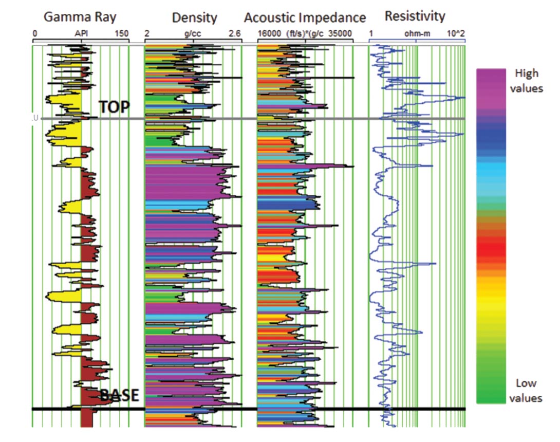
Acoustic impedances of sandstones and shales were found to be very similar, hindering the reservoir identification using only acoustic impedance. Figure 3 shows the segments of density, Gamma Ray, resistivity, and acoustic impedance log curves from a producing unit seen on a representative well. The well logs show the heterogeneous distribution of interbedded sandstones and shales within the reservoir and their density, acoustic impedance, and resistivity responses. The density vs. acoustic impedance (AI) crossplot (Figure 4) shows that density is an effective lithological indicator at the reservoir level: sandstones (green samples enclosed by the black circle) have lower density values than shales. According to these results, a multiattribute density inversion turns out to be a very good option for an effective reservoir characterization.

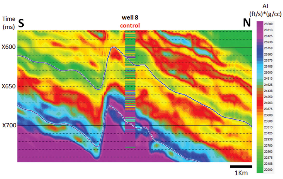
Despite the unpromising acoustic impedance properties of the reservoir, acoustic post-stack inversion was conducted to include the acoustic impedance volume as an input in the multiattribute analysis. Figure 5 shows the inversion results. The good correlation between the result of the seismic inversion and the acoustic impedance log is evident, in spite of the poor resolution showed by the inversion. In this area, most reservoir sandstones are below the seismic resolution (70 ft. approx.). In addition, López and Aldana (2007) state that sandstones have poor lateral continuity. This fact complicates the reservoir mapping.

Spectral decomposition

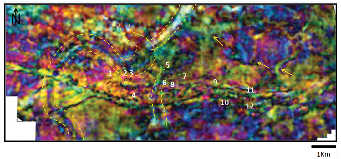
A spectral decomposition analysis was performed trying to map the reservoirs channels and heterogeneities described in previous studies of the area (e.g. López and Aldana, 2007). Using RGB images and numerous frequency combinations, we could observe several frequency anomalies with particular geometries.

The 35-45-55Hz RGB image, corresponding to a horizon slice shifted 30ms above the reservoir base (Figure 6), shows stratigraphic features oriented parallel to the sedimentation direction (S-N). Features located to the NE part of the study area show high amplitudes for 35 and 45Hz (yellow), and those to the West and South sides of the map, show purple to black anomalies, related to higher frequencies (55Hz). The frequency response could be associated to the thickness of the units. Giroldi et al., (2005) have related low frequency anomalies to large thicknesses, which implies that, possibly, these channels located to the NE are thicker than the ones located to the South and West of the area.

Since the spectral analysis of the seismic data was able to show geobodies and features related to lithological information of interest, frequency volumes of 20, 25, 30, 35, 40, 45, 50, and 55 Hz were included into the multiattribute analysis to generate the transform.

Multiattribute analysis

As mentioned before, the main goal of multiattribute analysis is to obtain an operator, linear or nonlinear, that can effectively predict log properties from neighboring seismic data at well locations (Hampson et al., 2001) and later extrapolate this relationship to the entire seismic volume. As seismic data and well logs have different frequency contents, in order to establish a relationship between them, we decided to apply a high-cut filter of 70-80 Hz to the density logs in order to filter high frequencies that do not exist in the seismic data.

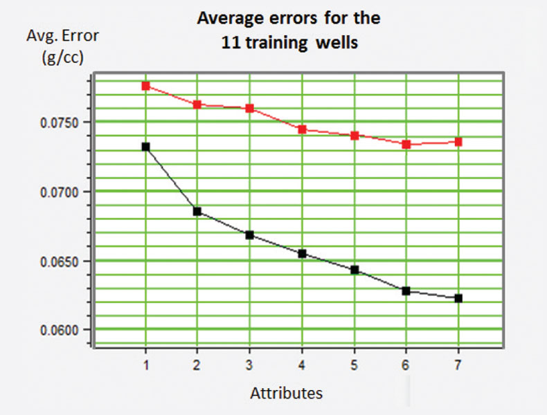
The multiattribute analysis comprises three main steps. First, a linear relationship between density and a subset of attributes is obtained using a stepwise regression to select the attributes that best predict the density log by minimizing the mean-squared prediction error between the original and the predicted target logs. The validation error for every attribute is also calculated. The validation curve tends to asymptotically decrease until one point and then begins to increase when the process overtrains (Hampson et al., 2001). When more than 6 attributes are included into the transform, the validation error increases, leading to erroneous density estimation at the locations where no log information is available (Figure 7). During this process, the stepwise regression automatically chooses the next attribute with the greatest contribution in an orthogonal direction to that of previous attributes. In this way, the linear independency of the attributes included in the transform is assured (Hampson et al., 2001).

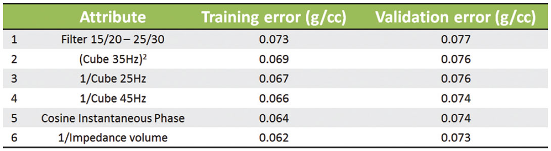
Table 1 shows the 6 attributes included in the multiattribute transform, based on the stepwise regression and cross-validation analysis. The normalized correlation coefficient for the multiattribute transform was found to be 0.58. It can be seen that frequency attributes, such as filters and frequency cubes, are the most statistically significant attributes for predicting density at well log locations. This suggests that the inclusion of the spectral attributes into the analysis was a good decision.

At second step, after finding the best linear combination of attributes, the determined linear transform is used for training the Multi-Layer Neural Network (MLFN) and Probabilistic Neural Network (PNN). The goal of training the neural networks is to find a nonlinear relationship that gives better results than those provided by the linear transform (Leiphart and Hart, 2001; Hampson et al., 2001 and Cedillo et al., 2004). The MLFN trained in this work comprises a set of neurons or nodes (processing units) arranged into three layers: an input layer, a hidden layer, and an output layer. The input layer contains as many neurons as the number of attributes to be included into the training. To determine the number of neurons in the hidden layer, several neurons were tried and those that give the least error between the original and the predicted logs were retained. The output layer has only one neuron since we are estimating one log.

Different neurons are connected between themselves by weights which are determined and updated by an optimization algorithm that minimizes the function error. PNN can be seen as an interpolation scheme that uses a set of measured variables to predict the value of an independent variable at locations where the measured variable is known.

Finally, the nonlinear transform that shows the highest crossvalidation is applied to the entire seismic volume. In this way a pseudo-density volume that allows an effective reservoir characterization can be obtained.

In figure 8 the cross-validation results of both, Multi-Layer and Probabilistic Neural Networks, are compared. The black log corresponds to the original density and the red log to the predicted density. The highest validation corresponds to the Multilayer Neural Network (0.52), which was used to obtain the pseudo-density volume.

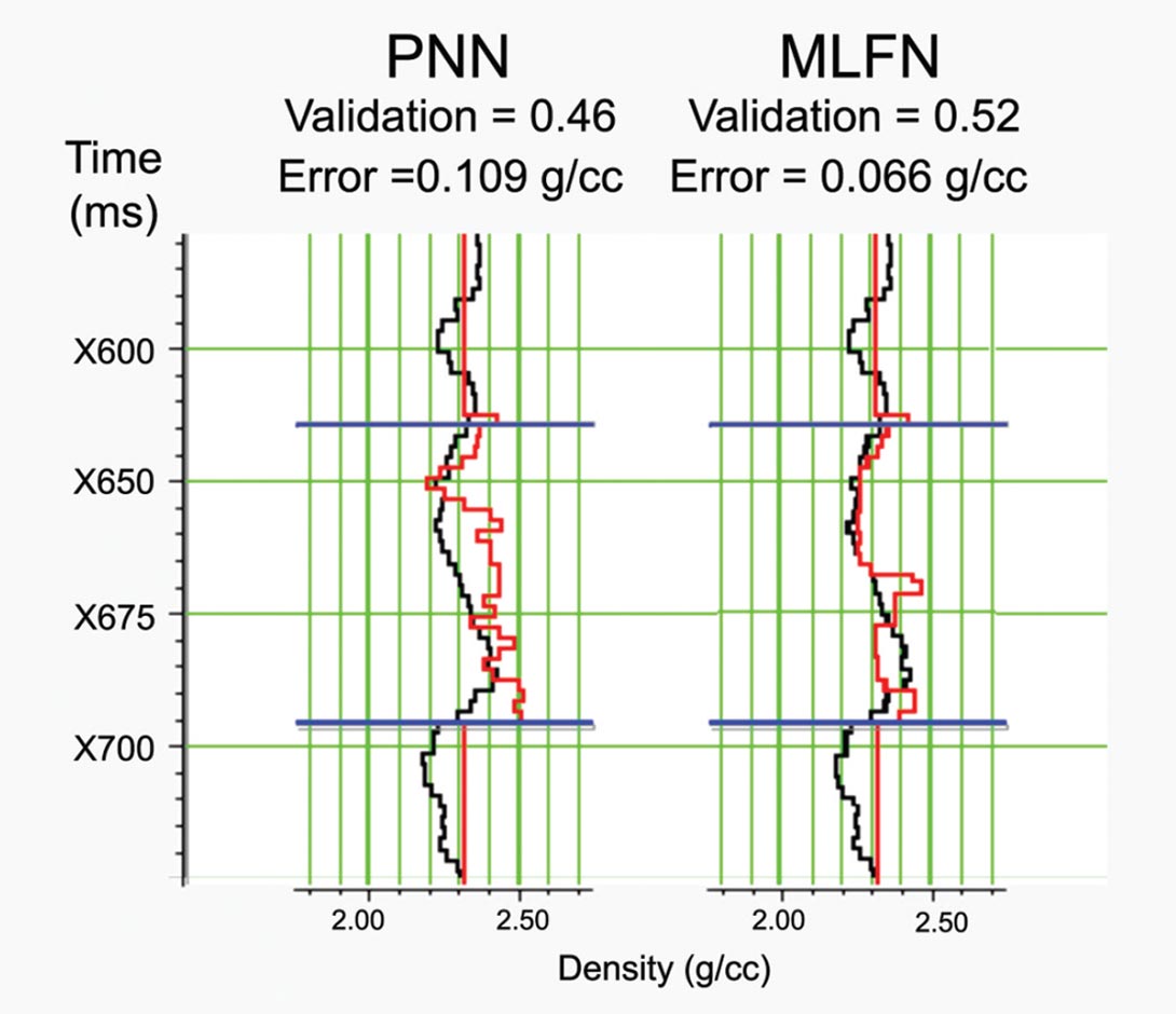
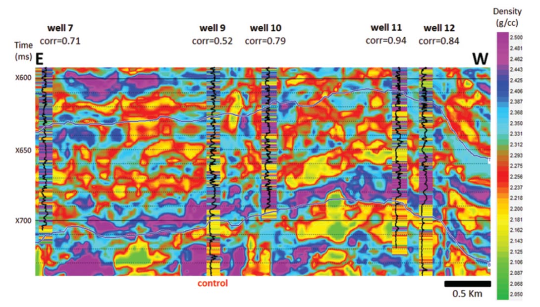
Figure 9 shows a seismic profile from the pseudo-density volume generated by applying the transform trained with the MFLN. This profile passes through wells 7, 9, 10, 11, and 12. There is a very good correlation between the pseudo-density volume and the Gamma Ray well logs with density as color scale. It is important to notice the good match between the control well (well 9) and the pseudo-density profile. This well was not included at any stage of the analysis in order to validate the performance of the transform in locations where no wells have been drilled.

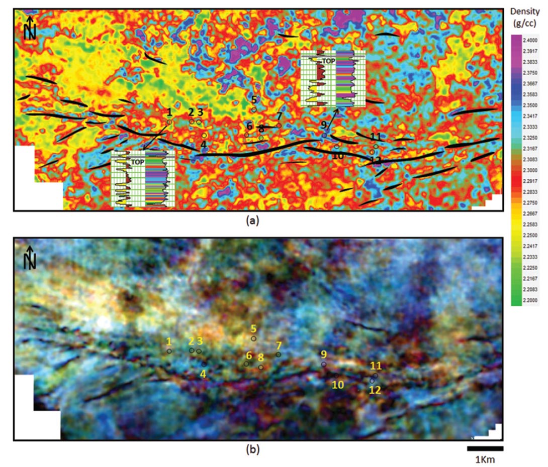
Average pseudo-density maps within 20ms interval above the reservoir base (Figure 10a) and within 20ms below the reservoir top were generated (Figure 11a). In the pseudo-density map at the reservoir base (Figure 10a), it is possible to observe anomalies, enclosed by yellow dotted lines, that allow identifying a possible channel with 35 and 45Hz dominant frequencies (light blue). Also an interesting geobody can observed to the NW of the area with 25 and 35Hz dominant frequencies (yellow). According to previous studies of the area (e.g. López and Aldana, 2007), this geometry could be related to deltaic environments. These features follow the orientation of the sedimentation direction (S-N).

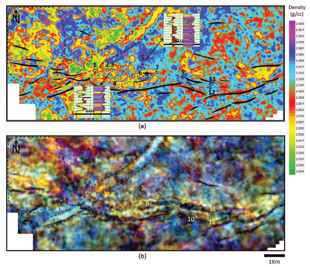
By comparing the pseudo-density maps with RGB images of 25- 35-45Hz corresponding to the same levels (Figures 10b and 11b), it can be seen that there is a very good match between them. Even a possible relationship between lithology and dominant frequency could be established: low density zones (sandstones) belong to areas with high amplitudes of frequencies of 25 and 35Hz (yellow zones in the RGB image). High density zones (major shale content) belong to areas with a dominant frequency higher than 45 Hz (dark blue and purple zones in the RGB image). It may be point out that these frequencies (25, 35 and 45Hz) were those included into the multiattribute transform by the stepwise regression technique.

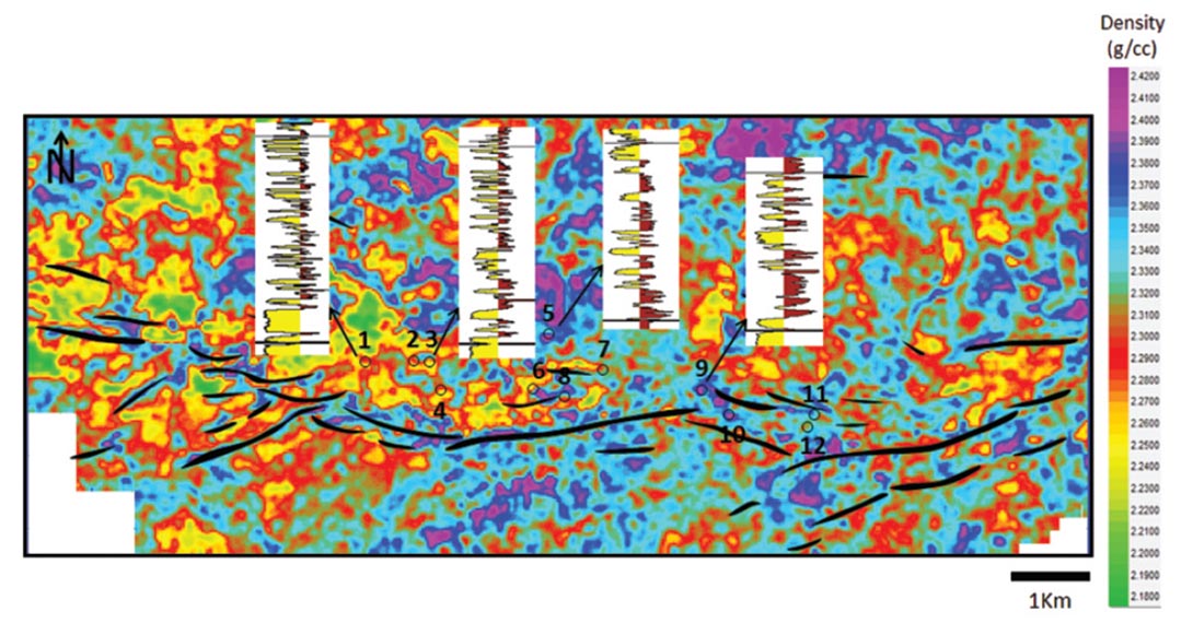
The heterogeneity of the reservoir, due to the combination of wave-dominated and fluvial sedimentary environments, can be observed in the pseudo-density map generated between the reservoir base and top (Figure 12). According to this map, the West zone of the study area presents higher sand content than the East zone. This observation is validated by the Gamma Ray logs superposed to the map. However, these logs also show that sandstones are thicker to the East than to the West zone. Information about production is needed in order to establish which zone has the best reservoir quality.

Conclusions

In this work, we have combined a spectral analysis and a multiattribute transform, trying to predict petrophysical parameters in order to characterize a heavy oil reservoir. The obtained results allow highlighting the significance of the application of geostatistical techniques, such as neural networks, to diminish the uncertainty during reservoir characterization. These techniques become particularly useful when analyzing reservoirs that have similar acoustic impedances between sandstones and shales, as the one studied here. In these cases, it is not appropriate to rely only on an acoustic impedance volume for characterizing the area.

Spectral decomposition analysis played a special important role in this work. The inclusion of this analysis as an input to obtain the multiattribute transform, allowed not only identifying interesting stratigraphical features, but also to establish an empirical relationship between dominant frequencies and lithological content.

Regarding the neural networks we have used in this study, a Multilayer (MLFN) and a Probabilistic (PNN), the MLFN provided more reliable multiattribute transform for density prediction in the study area than the PNN. This could be due to the training well’s sample interval (2ms; 10 ft aprox.), as the PNN is more sensitive to the amount of training data than the MLFN, and requires a representative training set (more training data) to achieve a good network performance.

Acknowledgements

We would like to thank William Marin for his support and collaboration during the development of this work.