AVO Modeling in Seismic Processing and Interpretation Part 1. Fundamentals

Introduction

AVO analysis is an effective technique in reservoir characterization and its success relies on not only the quality of recorded seismic data but also data processing and understanding of rock physical properties. Since AVO modeling is able to link rock properties to offset-dependent amplitude responses, it is a tool in assisting data processing, data calibration, and interpretation. This paper attempts to provide an insight in the current applications of AVO modeling. Part 1 of this paper reviews and discusses AVO modeling fundamentals: rock physical properties, AVO equations, AVO attributes and their relationships. Some issues related to AVO interpretation such as thin-bed tuning and offset-dependent tuning as well as fluid factor responses to fluid and lithology are specifically addressed. Part 2 will focus on AVO modeling methodologies and their advantages and limitations. Part 3 concentrates on the applications of AVO modeling in data processing, calibration and interpretation.

Seismic Rock Properties

Seismic rock properties are directly responsible for seismic wave propagation and seismic responses. They may be cataloged as basic rock properties (P-wave velocity, S-wave velocity and density, P- and S- impedance, Vp/Vs ratio and Poisson’s ratio), modulus rock properties (bulk modulus K, shear modulus μ, Lamé constant λ and ratios such as λ/μ ratio), and anisotropic rock properties (directional dependence of seismic velocity).

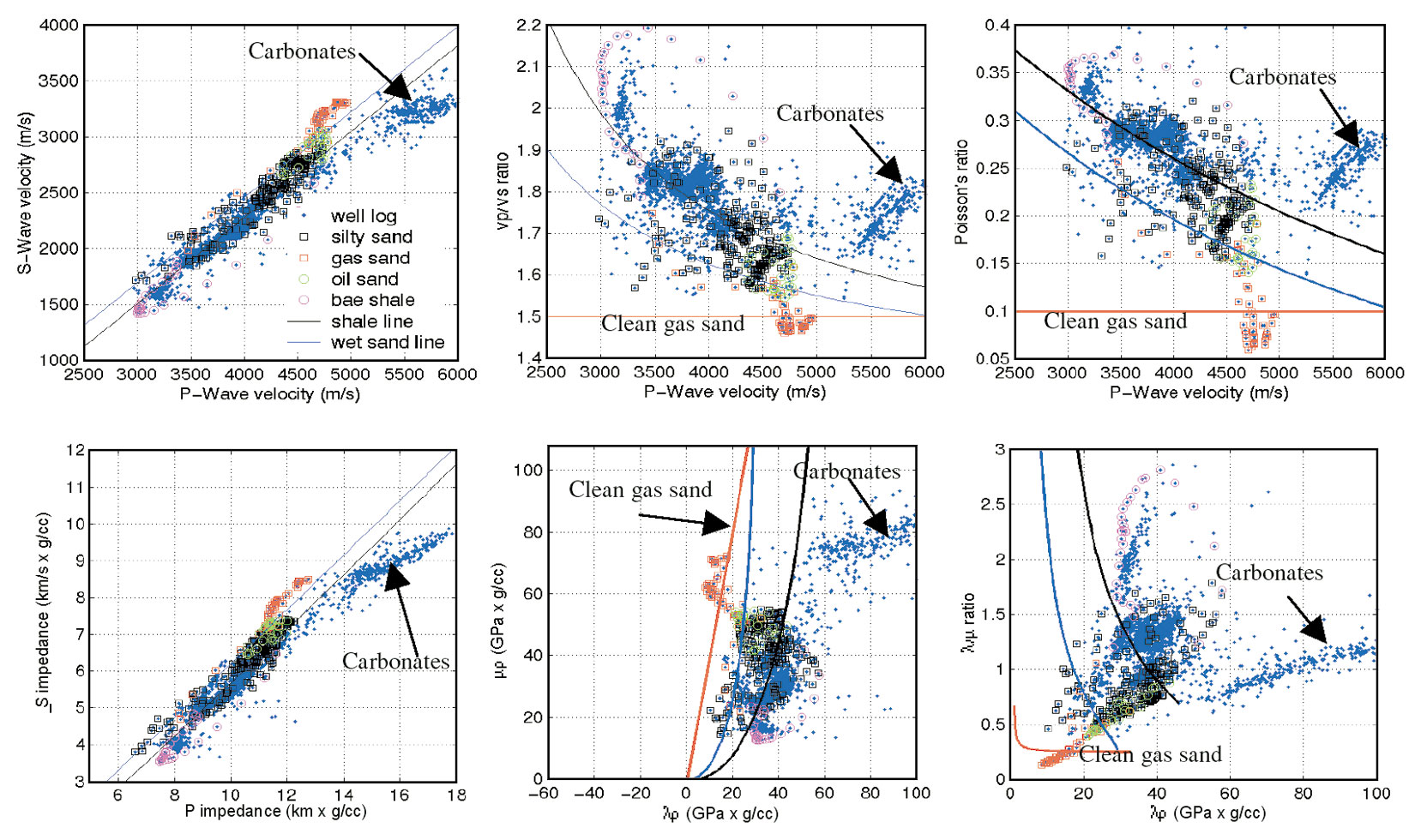
Various rock properties are calculated from a well in the Western Canadian Sedimentary Basin (WCSB) and cross-plotted (Figure 1). The overlain empirical relationships are shale (solid black), water saturated sand (solid blue), and gas charged clean sand (red). This is a gas well with gas-water contact. It can be seen that the velocities and impedances do not provide definitive discrimination as to whether the reservoir is a gas charged. However, Vp/Vs ratio, Poisson’s ratio, λρ, and λ/μ ratio for a gas charged reservoir have low values and better contrast to the encasing rocks. As we know, fluid has little effect on the rock’s shear modulus. Therefore, shear modulus is considered as reference information that reflects the properties of the rock matrix.

Usually petrophysical evaluation is the first step in any modeling project. The petrophysical rock properties that directly relate to seismic rock properties are volume fractions of mineralogies, porosity, and water saturation. A comprehensive description for deriving Vsh, PHIT (total porosity), PHIE (effective porosity) and SW from well logs was given by Elphick (1987). Fluid type, gas and oil ratio (GOR), oil and gas gravity (in API) and brine salinity (in ppm) are another set of important petrophysical properties. Fluid properties can be calculated based on calculated or in-situ measured pressure (P) and temperature (T) (Batzle and Wang, 1992). Predicting seismic rock properties, especially shear wave velocity, using petrophysical rock properties is an important task in rock physics. The steps for a typical seismic rock property prediction usually involve determining in-situ conditions, and calculating properties of fluid, properties of solid, and finally the seismic rock properties. The link between seismic rock properties and petrophysical rock properties can be clearly seen from Gassmann equation (Gassmann, 1951)

and

where K_dry = effective bulk modulus of dry rock; K_sat = effective bulk modulus of the rock with pore fluid; K₀ = bulk modulus of mineral material making up rock; K_fl = effective bulk modulus of pore fluid; ϕ = porosity; μ_dry = effective shear modulus of dry rock; and μ_sat = effective shear modulus of rock with pore fluid. In equation (1), K₀, ϕ, and K_fl are often calculated directly from petrophysical logs.

Numerous empirical relationships for seismic rock properties have been published and they are useful when either petrophysical properties are not available or rock physics theories do not meet the complexity of rock properties. Commonly used empirical relationships include the P- and S-velocity linear relation – also called mudrock line for clastics (Castagna, 1985), Han’s velocity-porosity-clay relation (Han, 1986), critical porosity model for K_dry (Nur et al., 1995), Greenberg- Castagna relation for mixed lithologies (Greenberg and Castangna, 1992), and empirical relations for carbonates (Li and Downton, 2000). The empirical relations often used by petrophysicists to derive sonic log or density log are Gardner’s density-velocity relation (Gardner et al., 1974), sonic and porosity relation (Wyllie et al., 1956), and resistivity-velocity relation (e.g., Faust, 1953). Above empirical relationships are useful but local relationships are strongly recommended as they reflect local variation of seismic rock properties. Calibration using available well logs may improve the predictions.

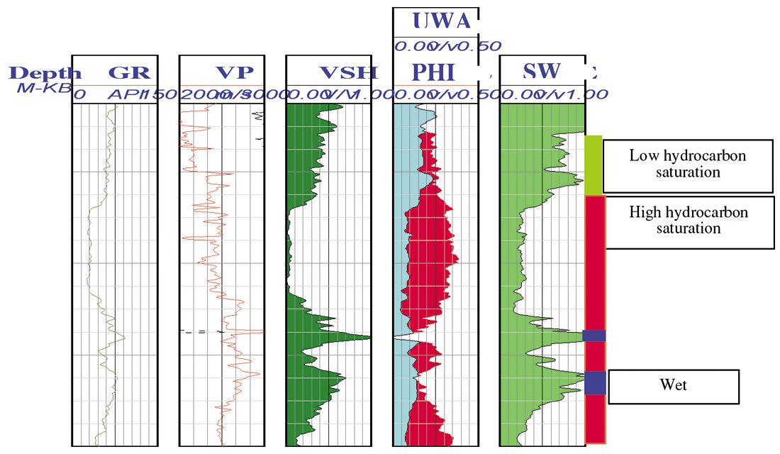
A set of petrophysical log curves from a WCSB well is shown in Figure 2. For this specific example, volume of shale is calculated as no carbonate or other mineralogies are involved at this well. The volume of shale, porosity, and water saturation are derived from resistivity, gamma ray, neutron density, and neutron porosity as well as local petrophysical parameters. Interesting observations from the petrophysical evaluation for this well include: 1) water saturation is proportional to Vsh; 2) gas saturation is opposite from 1), that is, gas saturation increases with decreasing Vsh; and 3) porosity increases with decreasing Vsh. One can also observe that clean sand has high gas saturation and dirty sand corresponds to low gas saturation. Further, notice that the cleanest sand still has a water saturation of about 25%.

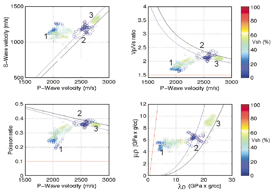
Figure 3 shows how volume of clay influences the seismic rock properties. It can be seen that clean sand is more sensitive to gas saturation. Also, the elastic rock properties of the oil saturated sand are similar to that of the brine-saturated since they fall on the empirical relationships of wet sand. Elastic rock properties together with porosity, lithology, lithology contrast are the sorts of things one can glean from petrophysics and rock physics analyses.

AVO Equations and Attributes

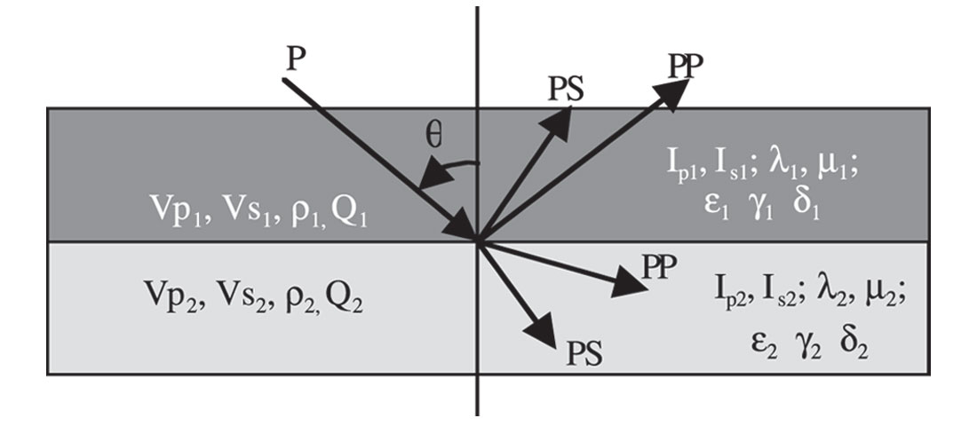
To illustrate the relationship between rock physical properties and seismic reflection, a two layer interface with incident P-wave and reflected and transmitted P-waves and converted S-waves is shown in Figure 4. The rock properties of the layers are P- and S-wave velocity, density, impedances, bulk modulus (K), shear modulus (μ), Lamè parameter (λ) and attenuation coefficient Q. The anisotropic properties are P-wave velocity anisotropic parameter ε, S-wave velocity anisotropic parameter γ and δ (Thomsen, 1986).

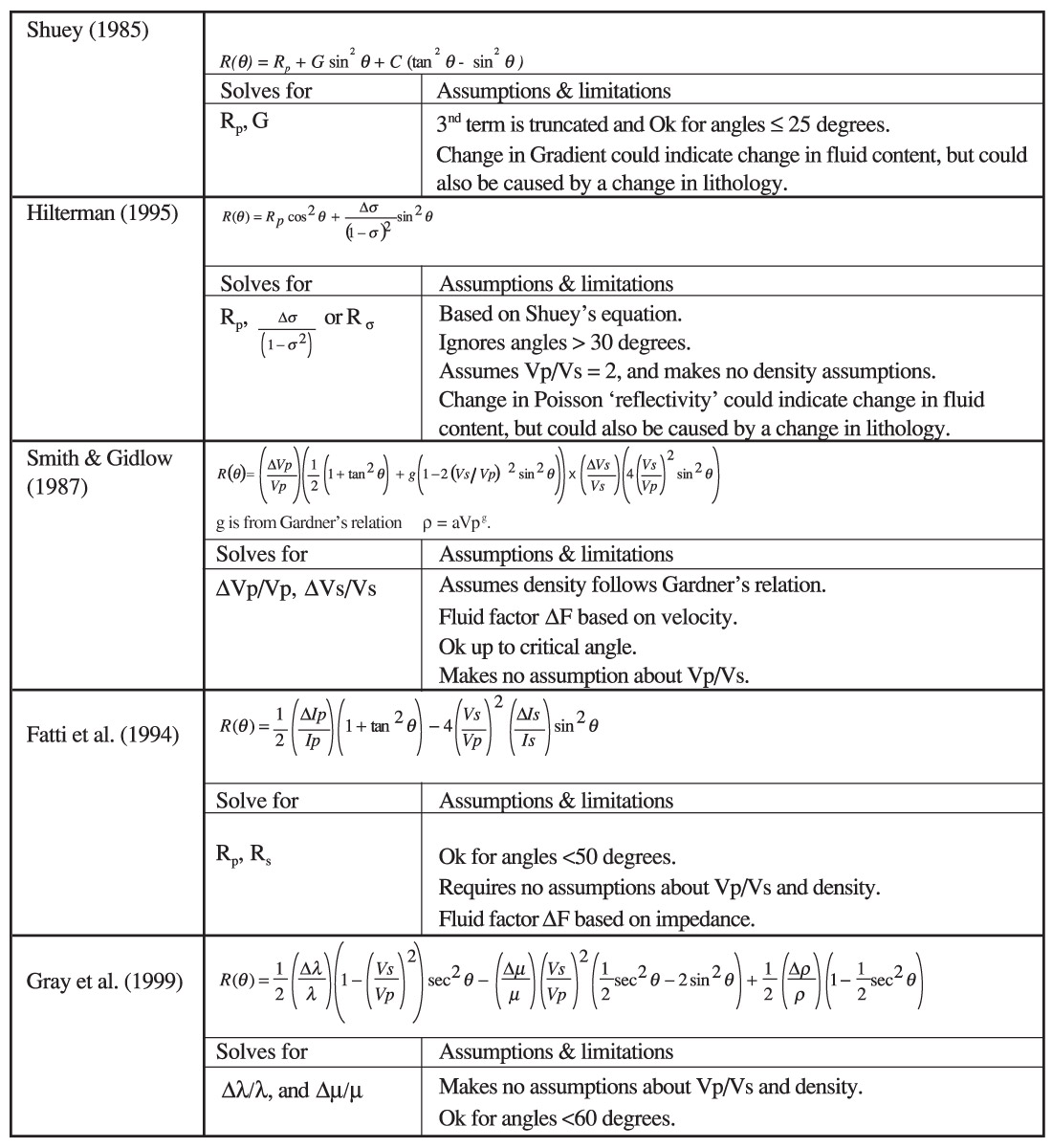
Zoeppritz equations describe the relations of the incident, reflected and transmitted compressional and shear waves at an interface of isotropic media. Zoeppritz equations and their approximation are often used in AVO modeling and data processing (Tables 1 and 2). Zoeppritz equations give the exact solutions but have complex forms. Aki and Richards (1979) gave the simplified forms of Zoeppritz equations. The difference between the exact solution and the solution from Aki-Richards’ approximation is small when the zero-offset reflectivity << 1. Re-arrangement of Aki-Richards’ equations is often used for describing and extracting AVO attributes that are considered meaningful for fluid and lithology indications. Commonly used P-wave equations are from Shuey (1985) for zero offset P-reflectivity R_p and gradient G, Smith & Gidlow (1987) for P- and S-velocity reflectivities, Fatti et al. (1994) for P- and S-reflectivities, Hilterman (1995) for P-reflectivity and Poisson’s reflectivity, and Gray et al. (1999) for Lambda reflectivity Δλ/λ and Mu reflectivity Δμ/μ. Fluid factor ΔF can be calculated from either P- and S-reflectivities or P- and S-velocity reflectivities (Table 3).

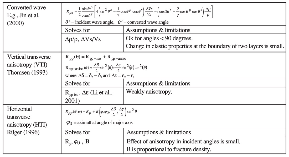
Converted S-wave equation (e.g., Jin et al., 2000), anisotropy equation for vertical transverse anisotropic medium (VTI) (Thomsen, 1993), and the equation for horizontal transverse anisotropic medium (HTI) (Rüger, 1996) are listed in Table 2. For converted waves, density reflectivity and shear wave velocity reflectivity or shear wave impedance reflectivity can be extracted (e.g., Jin, 2000). A more rigorous approach can be taken in solving P-wave, S-wave and density reflectivity by using simultaneous P-P and P-S inversion (Larson, 1999). Including both converted waves and P-P waves in the AVO inversion has the potential to make the estimate of density reflectivity more stable. However the issue of different wavelets and “event collaboration” must be addressed in order to realize this. Few efforts have been made in AVO attribute extraction for VTI media except some tested results (Li et al., 2001). The difficulties are in the simplification of an anisotropic AVO equation that requires reducing the number of terms from five to no more than three. For HTI medium, two-term Rüger’s equation with elliptical assumption for the amplitude is often used and the attributes to solve are fracture orientation and fracture density.

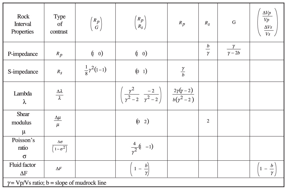
The definitions for commonly used attributes and their relations are given in Table 3. Some of these relations are exact and others are approximations. We may see that R_p can be calculated from R_s, gradient can be calculated from R_p and R_s, and fluid factor ΔF is calculated from R_p and R_s or ΔVp/Vp and ΔVs/Vs. Notice that the fluid indicators, gradient, fluid factor, and Δλ/λ increase with decreasing Vp/Vs ratio.

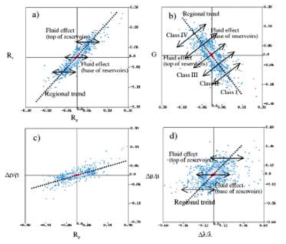
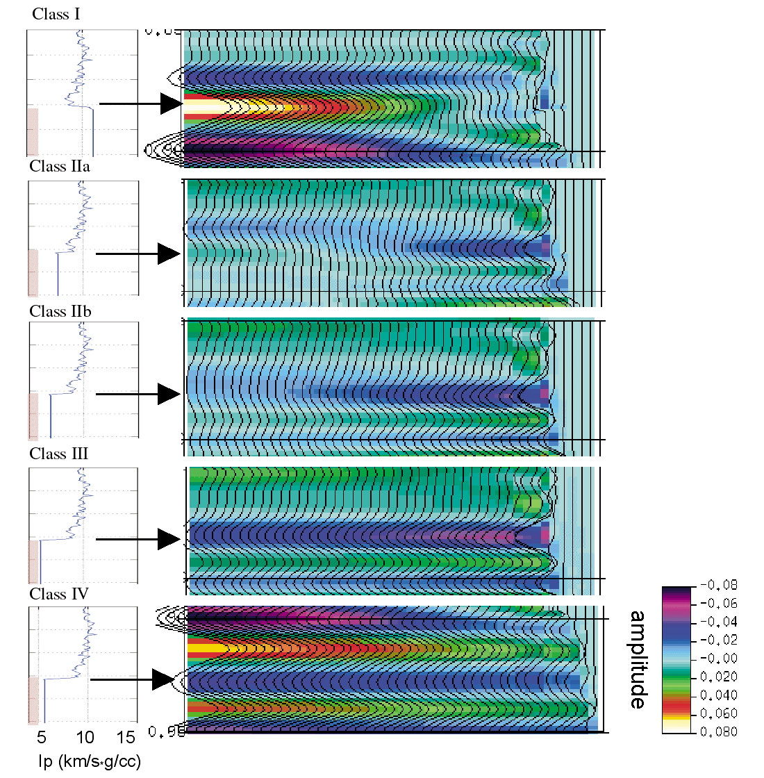
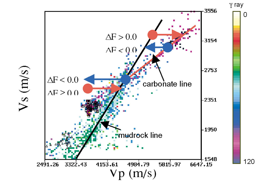
Cross-plots for the AVO attributes calculated from a dipole sonic log are shown in Figure 5. The dashed lines highlight the background trends. The arrows show the direction of the data points that shift when brine is replaced by gas or oil in rocks. The background trends of seismically derived R_p and R_s may differ from the trend calculated from well logs because of the influence from data processing. A calibration or correction can thus be performed. Figure 5b shows the cross-plot of R_p and gradient G. The types of AVO (Class I to IV) (Rutherford and Williams, 1989; Castagna, 1998) for a gas charged reservoir can be determined in this cross-plot space. An R_p and density reflectivity cross-plot is shown in Figure 5c. This information may be useful to those interested in extracting density reflectivity when it is considered more robust than other attributes in discriminating lithologies, such as in oil sand plays in WCSB (Downton, 2001; Dumitrescu et al., 2003). In Figure 5c, density reflectivities are small in comparison with R_p. In Figure 5d we can see that Δμ/μ and Δλ/λ have a magnitude approximately twice of R_p or R_s. In collaboration with Figure 5a, the synthetic gathers corresponding to AVO class I to IV are shown in Figure 6. It can be seen that class I AVO corresponds to high impedance gas sands. The top of the reservoir corresponds to a peak that deceases with offset and can change polarity at far offset. Class II AVO corresponds to a near-zero impedance contrast. The top of the reservoir corresponds to a weak peak or trough that may increase or decrease with offset. Class III AVO corresponds to lower impedance gas sands. The top of the reservoir corresponds to a trough that brightens with offset. Class IV AVO corresponds to lower impedance gas sands. The top of the reservoir corresponds to a trough that dims with offset.

Fluid factor is a commonly used hydrocarbon interface indicator. It is calculated by weighted difference between R_p and R_s as illustrated in Figure 5a. Gas-charged clastic zones will deviate from the background trend and display in fluid factor as a trough followed by a peak (blue over red in the usual fluid factor colour display). Except fluids, lithologies that do not follow the Vp and Vs relationship for brine-saturated clastics may produce a fluid factor anomaly. For example, coal produces an anomaly similar to gas sand reservoir. Carbonate manifests itself as fluid factor anomaly but does not follow the criteria of clastic rocks. For carbonate encased by lower impedance clastic rocks, we expect to see a fluid factor peak followed by a trough (red over blue in the usual fluid factor colour display). Ideally, a carbonate ‘mudrock line’ should be used in identifying a carbonate reservoir. In reality it is rather difficult to implement. For more complex cases such as multi-layer inter-bedded carbonate and shale, fluid factor anomalies become complex to interpret and thus care must be taken. In addition, fluid factor response may appear as a single peak or a single trough when the reflection at the top or base of a reservoir is not well developed for an anomaly.

To demonstrate AVO attributes in seismic wiggle trace form, a synthetic cmp gather with a low impedance reservoir is generated and the attributes are extracted based on the equations listed in Table 1 (Figure 8). The reservoir produces a Class III AVO anomaly. The extracted attributes from the cmp gather are compared with the same attributes calculated directly from well logs: the ‘reference’ attributes. The difference of the extracted attributes to the reference attributes is mainly due to offset dependent tuning, NMO stretch, the angle range that is used in AVO extraction, and theoretical approximations introduced.

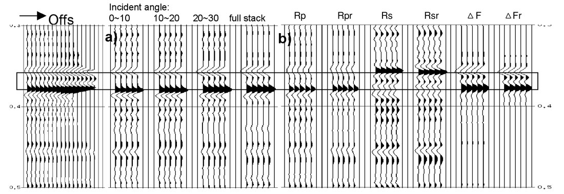
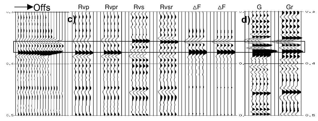
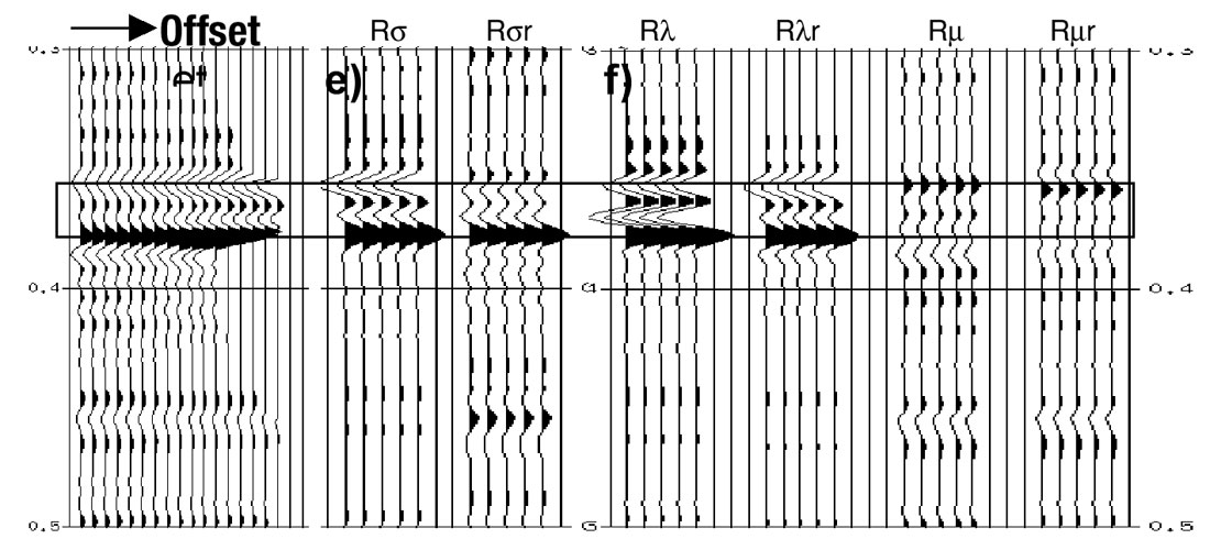
Figure 8a shows the angle-limited stacks. Notice that the stack with the angle range from 20 to 30 degrees has greater amplitude for both the trough and the peak. It also can be seen that the full angle stack is different from the zero-offset stack R_p in Figure 8b. This is a good reason to use the zero-offset P-reflectivity extracted from cmp gathers rather than a (full offset) structure stack as input to impedance inversion. For this example, inverting the full offset stack would give too-low impedance and an overly optimistic prediction of porosity.

P-reflectivity and S-reflectivity extracted using Fatti’s equation are shown in Figure 8b. We can see that the trough of P-reflectivity corresponds to the top of the reservoir. However, S-reflectivity is a peak as the reservoir has high S-impedance. As expected, the trough and the peak of the fluid stack correspond to the top and base of the reservoir, respectively.

The attributes extracted using Smith & Gidlow’s equation are shown in Figure 8c. For this specific example, ΔVp/Vp, ΔVs/Vs are similar to those attributes extracted using Fatti’s equation, telling us that density and velocity may follow a relation similar to Gardner’s (1974).

Gradient extracted using Shuey’s equation is shown in Figure 4d. It can be seen that the negative gradient corresponds to the top of the reservoir and the positive corresponds to the base of the reservoir, which indicates an increasing of amplitude with offset.

Figure 8e shows the Poisson’s reflectivity extracted using Hilterman’s equation.

The last panel (Figure 8f) shows the Δλ / λ and Δμ/μ extracted using Gray’s equation. They were scaled by 0.5 for the purpose of having a similar amplitude range as the other stacks. We may see that Δλ / λ has strong trough and peak at the top and the base of the reservoir, respectively.

Tuning

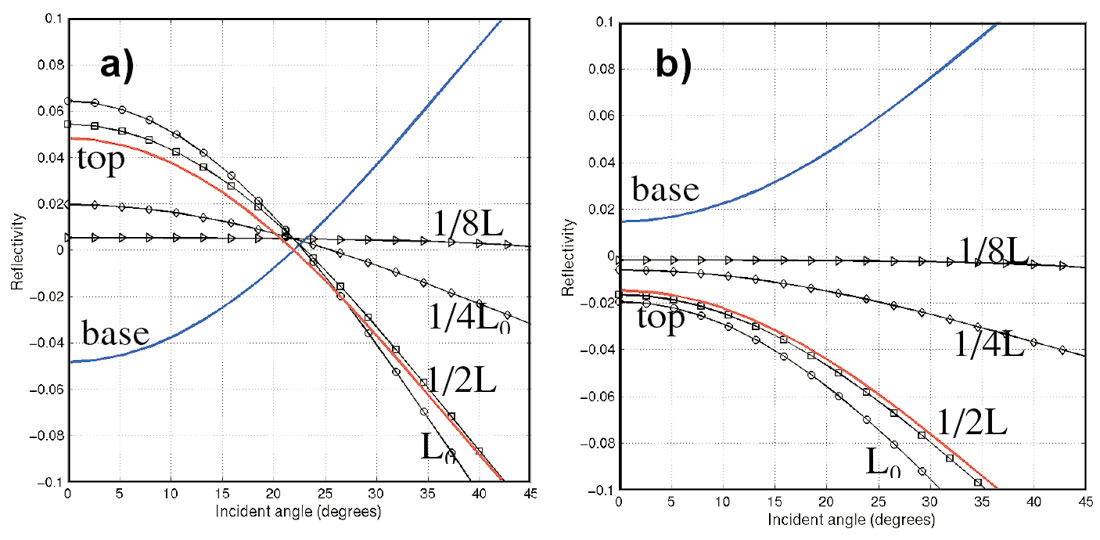
As we know, tuning has a significant impact on seismic resolution (Widess, 1973; Kallweit and Wood, 1982; Chung and Lawton, 1995). In AVO analysis, two types of tuning need to be considered: tuning due to thickness of a reservoir and offset-dependent tuning due to amplitude variation with offset. Both affect true AVO expression of an interface (Lin and Phair, 1993; Bakke and Ursin, 1998). Offset dependent tuning can be further affected by the differential travel time of adjacent reflections. It is important to notice that tuning may mask or induce an AVO anomaly. The offset (or angle of incident) dependent P-wave reflectivity for two adjacent Ricker wavelets can be expressed as

where A₁ and A₂ are the zero-offset reflectivities that correspond to two adjacent interfaces. Indices p and i represent primary reflection and the interfering reflection, respectively. θ_p and θ_i are the incident angles at the upper and lower interfaces. b is the thickness of the layer and L₀ is the wavelength of dominant frequency. Examples of Class I and III AVO anomaly and their tuning effects, for a reservoir with Vp = 3674 m/s and Vs = 2055 m/s, are calculated and shown in Figure 9, where red and blue lines represent the reflection from the top and the base of the reservoir without tuning. The top reflection interferes with the base reflection with ratio of b/L₀ equal to 1, 1/2, 1/4, and 1/8. For both cases there is a significant change in the amplitude when the b/L₀ equates to 1/4 and 1/8. From this example, we can see that when quantitative AVO analysis is performed on reflectivities that suffer from tuning, the AVO attributes, in turn, will be inaccurate.

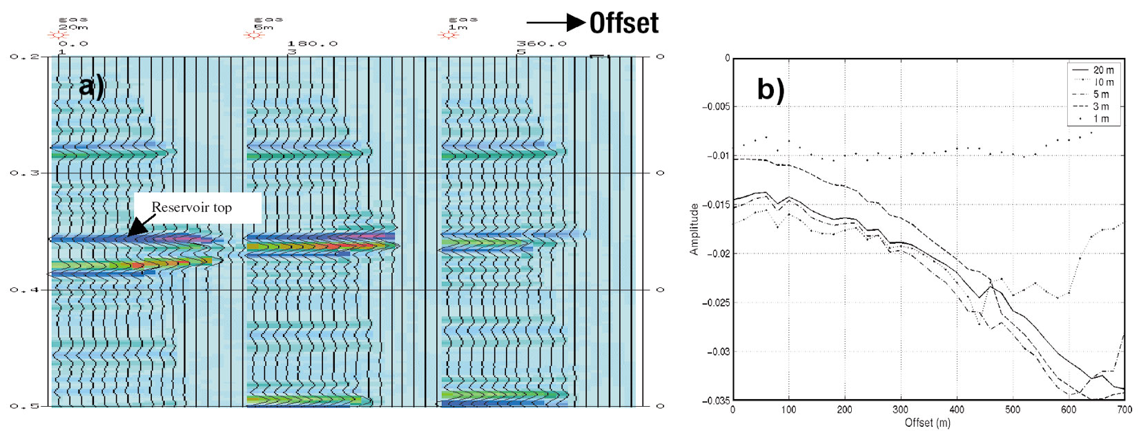
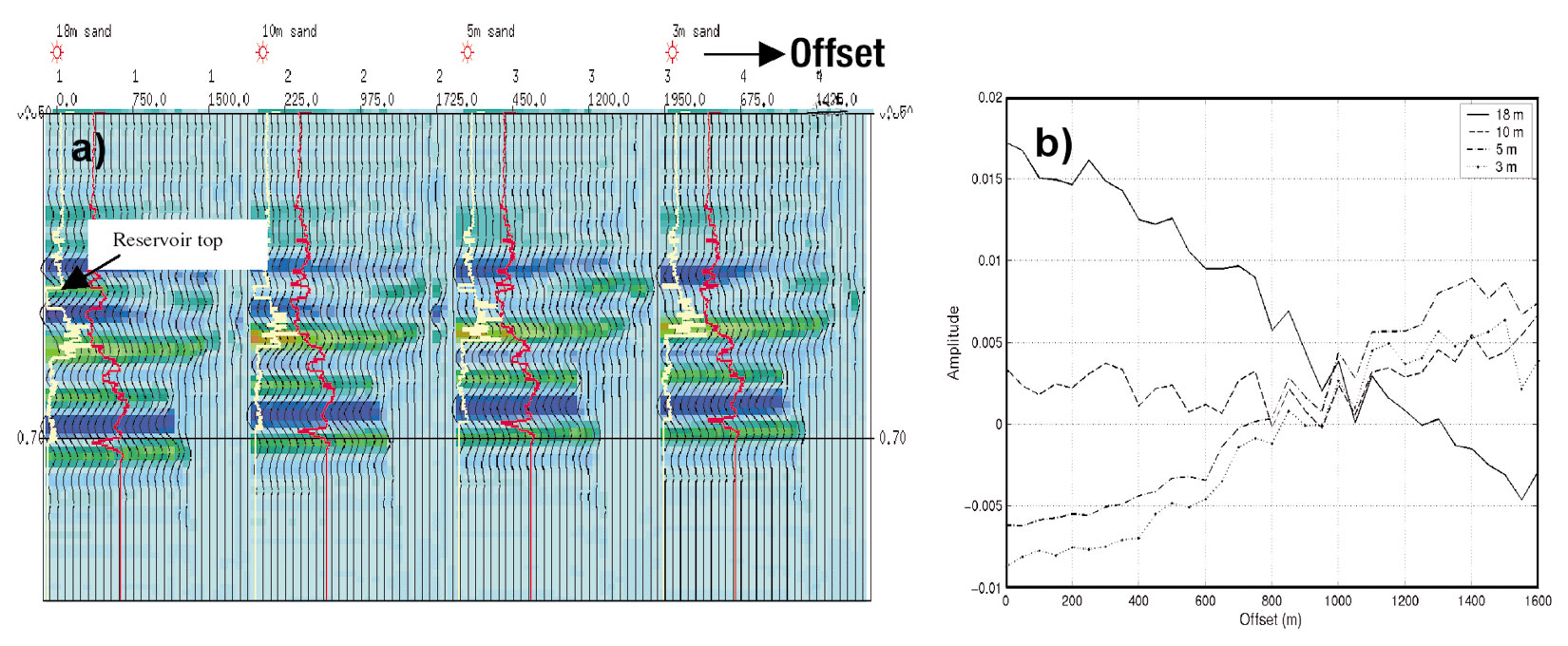
To further demonstrate the tuning effect, synthetic cmp gathers with Class I and Class III AVO anomalies are generated using well logs. The Class III AVO anomaly is from an unconsolidated gas sand with an average P-wave velocity 1900 m/s (Figure 10). The frequency bandwidth used is 8/14 – 90/100 Hz. Due to the low velocity of the reservoir, a Class III AVO anomaly can still be observed when the thickness is 5m. The amplitudes from the top of the reservoir corresponding to different thickness are shown in Figure 10b. A dramatic change in amplitudes occurs when the thickness is reduced to 1m. The Class I example is a tight gas sand with an approximate interval velocity 4600 m/s (Figure 11). The bandwidth for this case is 10/15 – 100/120 Hz. When the gas sand has a thickness of 18m, the Class I AVO response is a peak at near offsets that dims with offset and then reverses polarity at far offsets. As the thickness is reduced, (Figure 11b) this Class I AVO anomaly becomes a completely different AVO response: a trough at near offsets becoming a peak at far offsets. As we know, similar effect may occur when the bandwidth is reduced. Therefore, both the frequency content in a data set and the thickness of a target reservoir are important in determining how successful an AVO analysis could be.

Conclusions

This article, Part 1 of AVO Modeling in Seismic Processing and Interpretation, reviews AVO modeling fundamentals including rock physical properties, AVO equations and AVO attributes. It emphasizes the influence of petrophysical rock properties on seismic rock properties. Tuning is specifically discussed to realize its importance in the resolution of pre-stack data. The aspects routinely encountered in AVO analysis, particularly the links between AVO responses and rock properties and interpretation of AVO attributes such as fluid factor have also been addressed.

Acknowledgements

The authors would like to thank Core Laboratories Reservoir Technologies Division for supporting this work. The author would also like to thank Bob Somerville, Huimin Guan, and Jan Dewar for their help.