AVO Modeling in Seismic Processing and Interpretation Part III. Applications

Introduction

AVO modeling plays an active role in three areas: new technology development, QC data processing, and assisting data interpretation. This paper attempts to discuss these issues, with emphasis on the applications of AVO modeling in data processing and interpretation. Data modeling is introduced for its theoretical background and its applications in isotropic and anisotropic situations. In the data processing side, we will focus on calibrations. Finally, some discussion is given on the applications of AVO modeling in interpretation with additional case studies.

AVO Data Modeling

In the pre-stack processing stage, the cmp gathers that are considered having appropriate amplitude recovery or having gone through true amplitude processing are modeled using AVO equations to solve AVO attributes. This can be called AVO data modeling. Using the AVO equations introduced in Part I of this article, data modeling is implemented on the amplitudes at a given two-way time of a cmp gather. This is often implemented using angles of incidence for a linear fitting, or, a surface fitting for cases where two variables, offset and azimuth for HTI media, are involved. AVO data modeling is usually conducted using least square s method (L2 norm) or other robust methods such as L1 norm. The difference between L2 and L1 norms is that L2 minimizes squared deviation and L1 minimizes the absolute deviation of the data from a model. L2 norm and L1 norm have the form of

and

Where

is the single data point residual and d(x_i) is the data and m(x_i) represents an AVO equation fitted at given offset or angle of incidence x_i. Since number of data points n or offsets is always greater than the number of variables or AVO attributes to be solved, this is an over-determined problem. Minimization of the norms results in the solution. For L2 norm, the matrix form of the minimization is a = (A^T· A )^-1· A^T· d, where a is AVO attribute vector, A is angle-dependent coefficient matrix formed by an AVO equation corresponding to angles of incidence, and d is the vector of data (amplitudes). For L1 norm, median of coefficient of an AVO equation may be used in minimization (Press et al., 1989). To stabilize the solution, constraints from rock physical relationships may be brought in. The solution often consists of two AVO attributes. Shuey’s equation, for example, yields intercept and gradient, and Fatti’s equation yields P- and S- reflectivities.

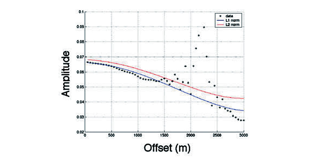
In the amplitude fitting, L2 norm is particular appropriate when the data contain random noise. L1 norm is considered robust when a small number of data points have deviant amplitudes, such as a multiple cutting across a primary reflection. To demonstrate L1 norm and L2 norm in AVO attribute extraction, a synthetic data set with strong coherent interfering noise was used and is shown in Figure 1. Fatti’s equation was used for amplitude fitting in this case. We can see that the L1 norm operation results in a better solution while the L2 norm solution is compromised by the spurious data points.

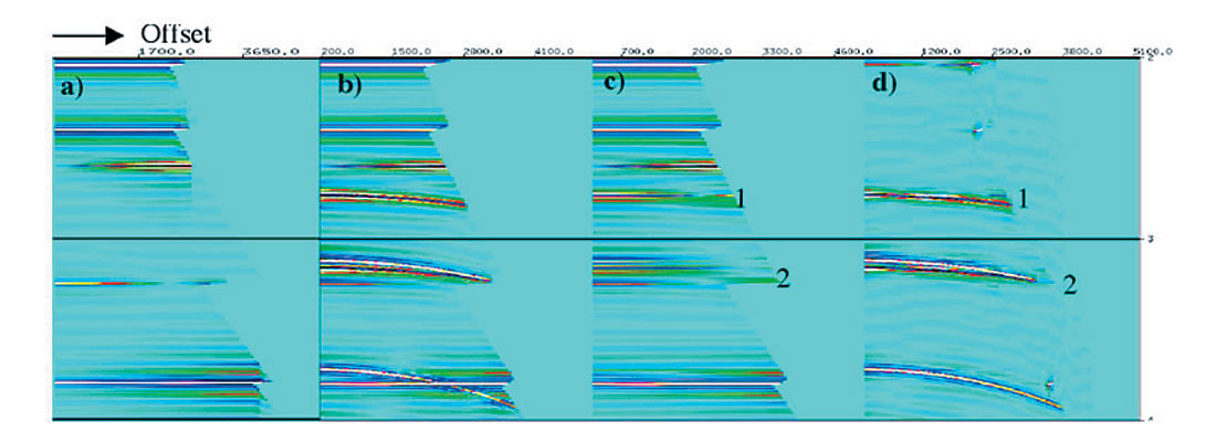
To further demonstrate this, a synthetic gather with primary reflections and multiples was processed through L1 norm solution of Fatti’s equation. Figure 2a to 2d are primary-only gather, input cmp gather, reconstructed gather from the extracted P- and S-reflectivities, and difference between Figure 2b and Figure 2c. As expected, The L1 norm solution does a good job in rejecting the large moveout multiples (the large moveout multiple is essentially gone from the reconstructed gather Figure 2c). Some energy from the small moveout multiples labeled 1 and 2 is still present on the reconstructed gather. Ideally, the reconstructed gather should contain only primary signal (Figure 2c should look like 2a). Hence, multiple attenuation may be required before AVO attribute extraction.

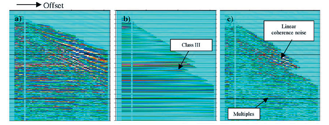
A real data example of AVO data modeling is shown in Figure 3. We can see that the input cmp gather (Figure 3a) contains random noise, linear coherent noise, and multiples. The input cmp gather (Figure 3a) is modeled by Fatti’s equation with L1 norm operation. The P- and S-reflectivities were solved and used in constructing Figure 3b. As indicated, the Class III AVO is successfully modeled. The random noise, linear coherent noise, and multiples are rejected and shown in Figure 3c. In practice, the difference gathers is used to examine if any reflections have been rejected due to poor NMO or inappropriate processing.

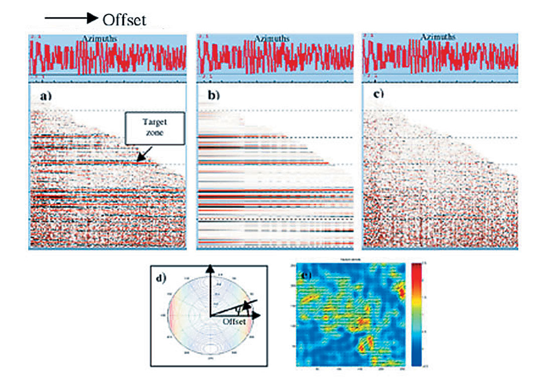
A second example is from a 3-D data set for studying AVO in a fractured reservoir. The fractured reservoir is considered as horizontal transverse isotropic (HTI) medium (Figure 4). For this case, L2 norm data modeling was performed based on Rüger’s equation (1996). To enhance the resolution and increase the stability of the data modeling, a surface fitting approach was taken to include all traces in the calculation. By examining Figure 4c, we see that the reflection events have been successfully modeled since little primary energy leakage can be seen. Figure 4d is a calculated theoretical amplitude surface that illustrates the amplitude variation with offset and azimuth. The resulting attributes in this AVOZ analysis are zero-offset reflectivity, fracture orientations, and gradients parallel and perpendicular to the fracture orientations. The fracture density is calculated based on the gradients. Figure 4e gives the estimates of fracture orientation and fracture density at a carbonate formation.

Data Calibrations

Calibration on cmp gathers and output AVO attributes can be conducted for optimizing AVO processing. It helps to answer the questions such as: whether the cmp gathers are properly processed with an amplitude friendly processing flow and parameters; whether phase, tuning, signal-to-noise ratio and other factors are influencing the solutions; and whether the correct impedance background is used in elastic rock property inversion. Calibration is often implemented by using well logs, synthetic gathers, walkway VSP, and/or known relationships between AVO attributes or between rock properties. Calibration can be performed locally at a cmp location, or globally on a data set.

Using synthetic cmp gather(s) to tie seismic often gives a quick insight to the data. AVO type and its variation are often determined in this stage. Further, since AVO modeling links seismic responses directly to rock properties, it helps to confirm or define reservoir condition. One may perturb the well logs to represent the possible reservoir conditions. For example, gas substitution may be performed on a wet well or vice verse. The other parameters that are often changed are porosity, reservoir thickness and lithology. Figure 5 shows an example in which a synthetic cmp gather ties to a recorded cmp gather. In the zone of interest, the AVO expression has similar character. We may therefore consider that the data has appropriate amplitude recovery.

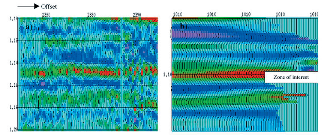
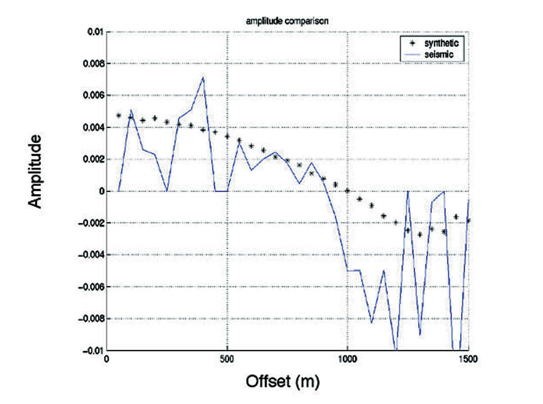
Calibration at specific reflections may be performed. The amplitudes for a given event from both the actual seismic and the synthetic can be extracted and compared. Figure 6 shows an example in which the seismic amplitudes from the top of a gas reservoir are compared with the synthetic gather. The Class I AVO anomaly with polarity reversal at the far offsets is confirmed as the AVO expression for this reservoir.

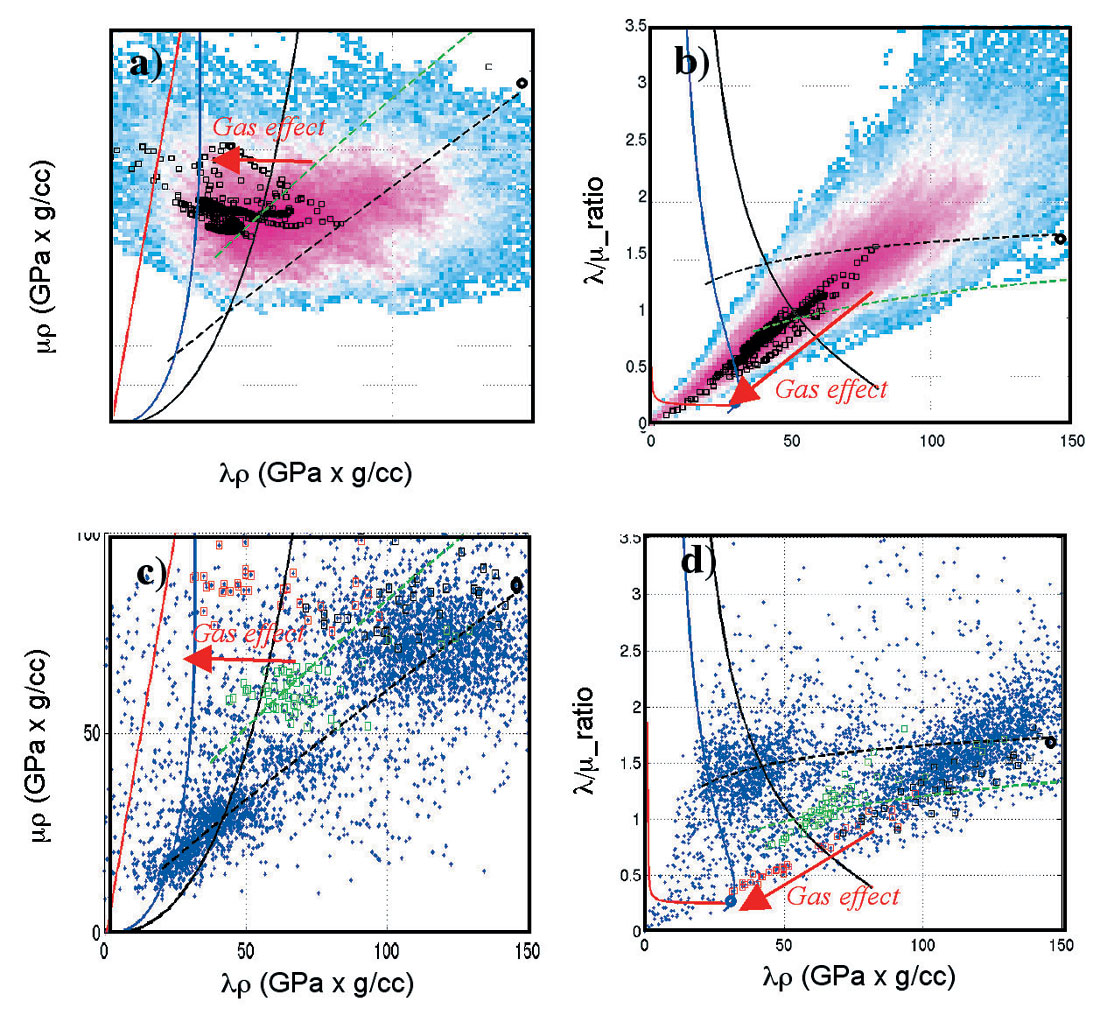
Further, calibration can be conducted on AVO attributes or inverted rock properties. P- and S-reflectivity synthetic may tie to stacked P- and S-reflectivity sections. It also can be conducted in cross-plotting spaces such as P-reflectivity against S-reflectivity, and λρ against μρ. Figure 7 shows an example using well logs to calibrate inverted elastic rock properties for a gas charged dolomite reservoir. In Figures 7a and 7b, the inverted elastic rock properties of the reservoir are highlighted in black squares. The overlain empirical relations are shale (solid black), water saturated sand (solid blue), limestone (dashed black), dolomite (dashed green), and gas charged clean sand (red). We can see that the data points from the gas-charged reservoir are shifted towards low λρ values and low λ/μ ratio. Figures 7c and 7d show the cross-plots of dipole sonic logs. The data from a gas charged dolomite reservoir are highlighted with red squares, and brine-saturated porous dolomite with green squares. This comparison leads to an interpretation of a gas-charged dolomite based on the seismically-derived elastic rock properties (Figures 7a and 7b). In addition, the porosity of the reservoir is similar to the porous dolomite that is highlighted by the green squares.

Global calibration implies a way to QC data on entire data set. For example, the amplitude variation with offset within a time window can be calculated and compared to that from synthetic gathers. Consequently, offset-variant scaling corrections may be applied to the data set. Calibration may also be conducted based on relationships of AVO attributes such as P- and S-reflectivities. Background constraints that are used in data modeling and elastic rock property inversion may also be calibrated through this method.

Interpretation

AVO modeling assists interpretation on cmp gathers, AVO attributes, and inverted elastic rock properties. It helps in validating AVO responses and linking seismic expression to known reservoir conditions. AVO modeling can increase confidence in interpretation and reduce risk in reservoir characterization as it provides independent information. We can use synthetic to identify AVO anomalies and determine AVO types on a cmp gather. Also, we can use synthetic pre-stack data to determine the S-wave information that often is ignored in conventional data processing. For instance, a strong S-impedance contrast may exist for a reservoir even though P-impedance contrast is small. The derived AVO attributes such as fluid factor, and inverted elastic rock properties such as Vp/Vs ratio, Poisson’s ratio, λρ and λ/μ ratio can be used to infer the fluid type in a reservoir.

Tuning may invoke or mask an AVO anomaly. The synthetics with varied bandwidth or reservoir thickness may give answers to tuning questions. Special lithologies or lithological contrasts may generate AVO anomalies and can be proved by AVO modeling. Lithological complexity may also bring in difficulties in interpretation. Tight streaks may manifest themselves as AVO anomalies and brighten in a stacked section. Coal, carbonate, and the lithologies that do not follow water saturated trend of rock properties for clastics may complicate fluid stack anomalies. The lack of understanding on some seismic rock properties may prevent one to effectively explore those types of reservoirs. Further, high clay content in sand may result in low gas saturation. This type of partial gas saturation may still have relative high Vp/Vs ratio that contradicts traditional theories of partial gas saturation. Therefore, AVO modeling may provide opportunities for distinguishing the partial gas saturated reservoirs based on the lithological effect on rock properties.

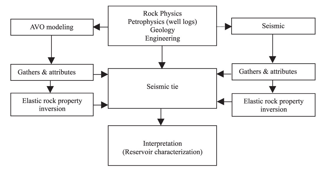
Figure 8 shows an ideal workflow in using AVO modeling to assist data processing and interpretation. We can see that AVO modeling workflow is the same as that of data processing. Therefore, seismic data and synthetics can be compared in the stages of cmp gathers, AVO attributes and inverted elastic rock properties. In interpretation, the information from all three branches can be integrated. The risk in reservoir characterization may thus be reduced since the interpretation is broadly based, involving understanding of seismic, rock physical properties and geology.

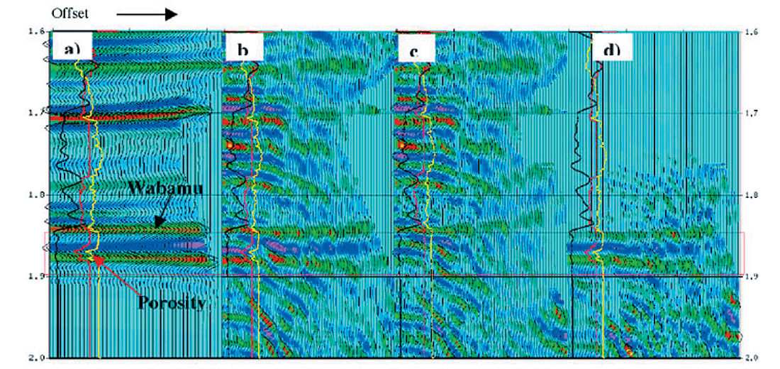
Several AVO modeling examples for AVO interpretation have been given in Part 1 and Part 2 of this article (Li et al., 2003; Li et al. 2004). Figure 9 shows an example using AVO modeling to understand interference of multiples and converted energy at the Wabamun dolomite porosity. The modeling was conducted using both 1) Zoeppritz modeling with ray-tracing, and 2) full wave elastic wave equation. For the elastic modeling, two cases were modeled: reservoir case (with porosity) and non-reservoir case (without porosity). The observations that can be made for this typical study include: a) Class III AVO anomaly (a trough brightens with offset) at the top of the reservoir presents in the Zoeppritz modeling but it does not show in the elastic modeling; b) the elastic modeling shows that multiples and converted energy (which are not accounted for in a Zoeppritz model) interfere with the reflections from both the top and the base of the reservoir; and c) the difference between the reservoir case (Figure 9b) and the non-reservoir case (Figure 9c) indicates that it could be enough for differentiating the porosity case from non-porosity case. Further, we may notice the inter-bedded multiples and converted energy generated by the reservoir (Figure 9d). This study provides the information of wave propagation and interference. We may use it as a guide for attenuating the coherent noise and performing amplitude recovery.

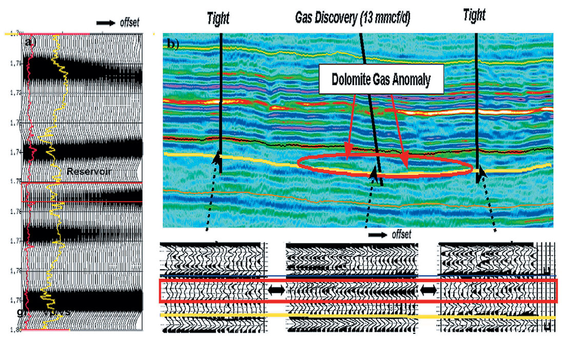
The second example is from a study on carbonate reservoirs (Li et al., 2003). In Figure 10a, AVO modeling shows that a gas charged dolomite reservoir produces a Class III AVO anomaly. This is consistent with the AVO response in the cmp gather at the location of the producing well. We can see that at the tight well locations, a completely different AVO response presents. The information provided by AVO modeling validates the information from seismic.

Conclusions

This paper, the third part of AVO modeling in seismic processing and interpretation, demonstrates some applications of AVO modeling involving data processing and interpretation. The discussion of data modeling provides an insight in AVO attribute extraction. Calibration using AVO modeling in data processing sheds some light on how to optimize AVO solution. Combined with rock physical property analysis, petrophysical analysis, and geological information, AVO modeling provides useful information in interpretation and thus increases certainty in reservoir characterization.

Acknowledgements

The authors thank Core Laboratories Reservoir Technologies Division for supporting this work.