Earth models are routinely used in the oil & gas industry to integrate multidisciplinary data for subsurface property predictions. While most earth models predict reasonably well at the field scale, they often fail to accurately predict the subsurface conditions at a specific location, especially in stratigraphically complex reservoirs.
There are ways of producing better predictive earth models. How? By integrating advanced 3D seismic information such as inversions, seismic stratigraphy and geomorphology into the model. Examples are used to discuss pitfalls and practical solutions for a successful quantitative seismic interpretation.
Introduction
Today, many resource plays are data rich, but many earth models still under utilize the data available. A classic example is the under utilization of information readily available from 3D seismic in building earth models.
After well to seismic correlation is established, a traditional seismic interpretation workflow would seek to establish a series of continuous time horizons using the normal suite of horizon picking options available in interpretation software packages. The historical techno-psychological objective for 3D seismic data has been to build continuous picked surfaces of specific correlated seismic reflections. These surfaces would then be used to guide inversions, provide stratigraphic level correlation to AVO and other attribute anomalies, constrain depth conversion process and so on. It has been a largely sequential, deterministic treatment of seismic data volumes. However, every interpreter knows there is ‘geology’ in the seismic data that is difficult to capture by such a process. A cursory 2D view of a 3D data volume, in either horizontal slice or vertical profile domains, typically shows geology: clinoforms, channels, variations in bed thickness and so on. The continuous horizon mapping approach minimizes the use of short reflection segments, whose dip, orientation, length, and distribution may all indicate aspects of the depositional or diagenetic environment. Earth modeling offers a means to quantify those types of qualitative, observational geological elements in the data.
Advanced interpretation workflows – such as seismic inversions, seismic stratigraphy and geomorphologic interpretations – are commonly performed by the geoscientist to extract indicators of reservoir properties from the seismic data. But these workflows are often run as standalone projects, and the information they yield is not typically incorporated into the earth model.
In the brief discussion which follows, various examples of clastic reservoirs are shown to demonstrate what type of information can be extracted from 3D seismic, and how it can be successfully integrated to build a more realistic and valuable earth model. The proposed methodologies are also applicable to carbonates and unconventional reservoirs.
Method
The way to quantitatively interpret seismic is to cross-validate it against geological and engineering data. So the first thing needed is to integrate as much data as possible with 3D seismic: a structural and/ or stratigraphic interpretation, well data (logs, core, image logs, dip meters...), engineering data (perforation and completion, production history, pressure, temperature...) and more. The use of geomodeling software is ideal since most commercial versions offer good integration capabilities with the required statistical and geostatistical tools for proper data investigation and modeling.
The cross-validation of seismic data against well data can be done either in time or depth. The most appropriate domain depends on the type of velocity information available (3D volume or at the wells only) and also on the software being used.
Inversion
Inversion is the process of transforming seismic reflection data into a quantitative rock-property description of a reservoir. It may be pre-or post-stack, deterministic or geostatistical. And it typically includes other reservoir measurements such as well logs, cores and a stratigraphic interpretation.
Post-stack inversion
Cross-plotting the seismic-derived P-Impedance with the well log derived P-Impedance is done in order to validate the inversion result. The well log derived P-Impedance first needs to be filtered to approximate the seismic frequency. A crossplot encompassing several hundred meters of depth should give a very high correlation coefficient since each stratigraphic unit will have different ranges of impedance values. When the cross-plot is restricted to data from the formation of interest, the correlation coefficient between the seismic and well impedance will most likely be lower than over a thicker interval (Figure 1), but it is often still good enough to be used to constrain an earth model. For example when the log derived P-Impedance correlates with the calculated well log porosity, and if it is confirmed that the seismic P-impedance correlates with the well P-impedance over the formation of interest, then the seismic P-Impedance can be used as a soft constraint in a porosity (and porosity dependent lithology) prediction using geostatistical methods.

Pre-stack inversion
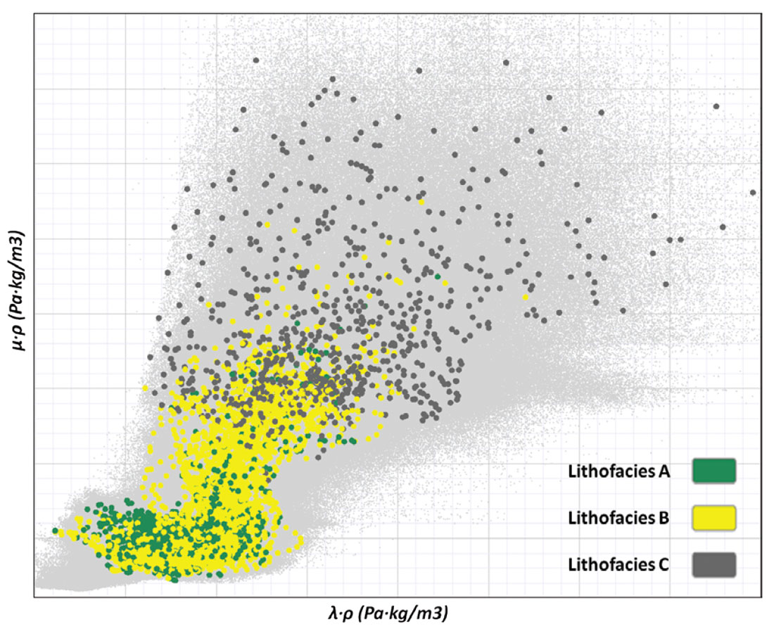
When interpreting a pre-stack inversion, and more specifically lambda-rho (LR) and mu-rho (MR) volumes, rock physics templates and deterministic cut-off lines in cross-plot space are often used to classify the seismic inversion volumes into lithofacies and fluids.
However this does not capture the inherent limitations of the classification process, as the lithofacies overlap due to the difference of scale between the seismic and the wells and to the uncertainty of the data itself (Figure 2).
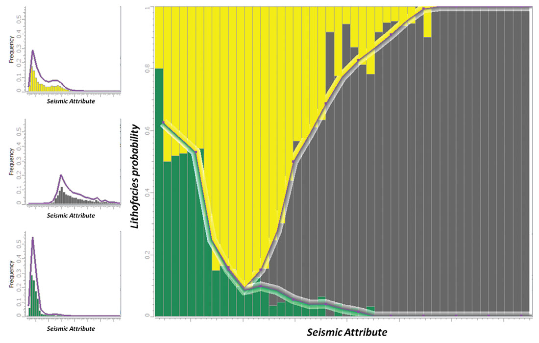
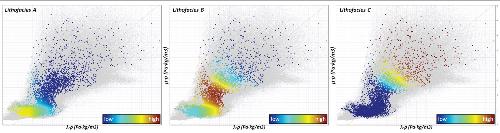
To address this issue, probabilistic calibration of each inversion volume (lambda-rho and mu-rho volumes, for example) is a more rigorous approach (Nieto et al., 2013). One way to do this is to calculate at the well locations a histogram of each seismic attribute for each lithofacies and then to normalize these into a calibration plot (Figure 3). The resulting lithofacies’ probability distribution functions are then statistically combined and can be displayed in the LR-MR cross-plot space for further analysis (Figure 4).
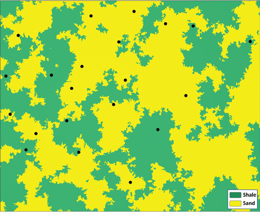
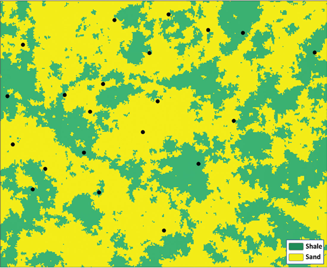
Once the seismic inversion volumes are properly calibrated to the wells, the resulting lithofacies probability volumes can be used as soft constraint in a lithofacies prediction using geostatistical methods. The example of Figure 5 shows how the use of seismic (in addition to the wells) influences the spatial distribution of sand and shale in an earth model.
Seismic stratigraphy
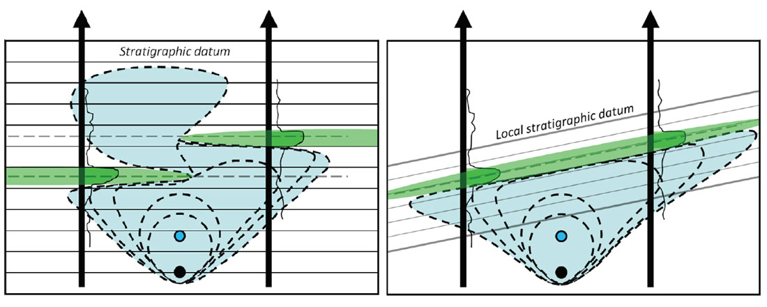
The stratigraphic layering in an earth model can strongly influence how wells can be correlated in three dimensional space within the model. For instance, two identical lithofacies on adjacent wells may or may not be correlated in the earth model depending on the inter-well stratigraphy (Figure 6). This uncertainty can have dramatic impact on reservoir performance prediction.
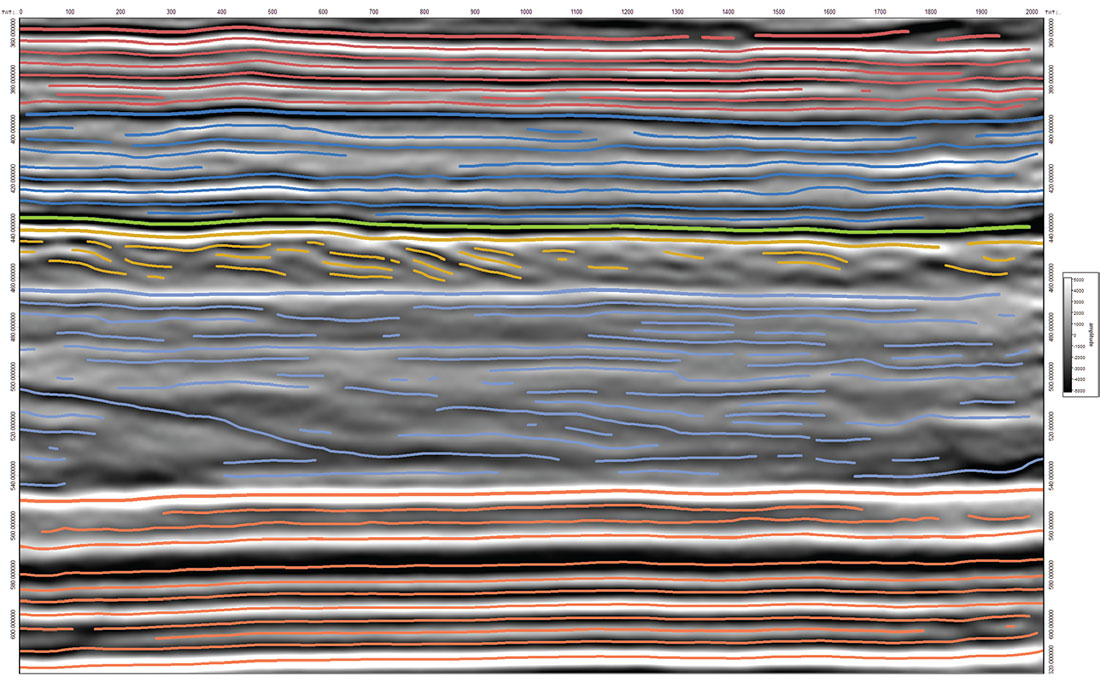
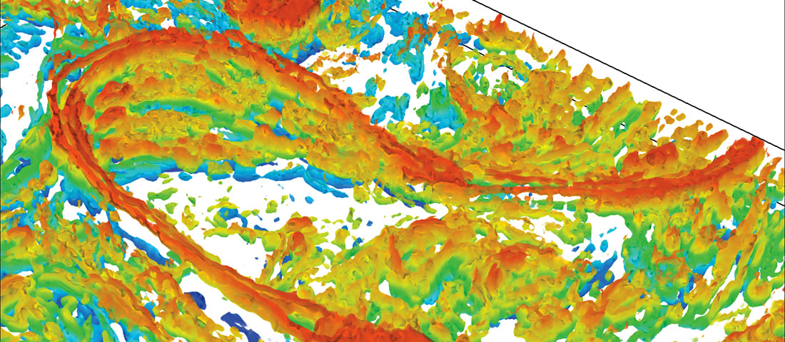
Stratigraphic trends can be interpreted using 3D seismic. In the McMurray formation (WCSB), for example, hundreds of small stratigraphic reflectors – discontinuous and spatially restricted reflection ‘fragments’ – can usually be interpreted over just a few square kilometers. Picking these reflectors manually would be extremely tedious and cannot be practically achieved. A better way is to manually pick seeds in areas of interest and then auto-track the stratigraphic reflectors. Even better is to use a fully automated stratigraphic auto-picker that can extract automatically almost every single reflector within a stratigraphic interval (Labrunye et al., 2013) as shown in Figure 7.
As with any automated process, it is important to check the validity of the extracted stratigraphic reflectors. The most convenient way is to slice through the entire model, displaying the stratigraphic trends as lines and the wells with lithofacies and stratigraphic markers, with seismic amplitude in the background. Visualizing the stratigraphic trends in 3D can also reveal interesting geomorphologic features.
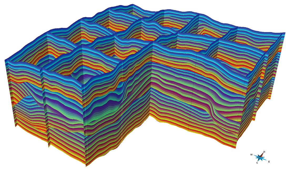
These local trends are then used to build a high resolution stratigraphic model (Figure 8). Additional types of data – 3D seismic attributes (dip and azimuth), dip meter data and stratigraphic well markers – can also be used to constrain such stratigraphic model. Previous work done by Bujor et al. (2012) have shown that the prediction of lithofacies within such high resolution stratigraphic frameworks produces more realistic lithofacies transition and continuity than within conventional top-down stratigraphic frameworks, and improves the predictability of the earth model. The high resolution stratigraphic models can also in turn improve the low frequency model of a model based inversion (Brouwer et al., 2012).
Seismic geomorphology interpretation
Seismic amplitude alone often carries a lot of information such as geomorphologic features. A combination of cross-sections and stratigraphic slices is the key to recognize geomorphologic patterns and to extract the associated geomorphologic features (Posamentier, 2005). The high resolution stratigraphic model discussed previously increases the chances of finding geomorphologic features. An example of fluvial channel interpreted from a 3D seismic using the high resolution stratigraphic model is shown in Figure 9.
There are several ways to extract the geomorphologic features, once identified. One commonly used approach is to pick geobodies (such as fluvial channels), geomorphologic trend lines (such as point bars) or discontinuities (boundaries). The next challenge is to successfully integrate this interpretation into an earth model. Once again there are several ways to do so. One approach is to split the earth model using deterministic geobodies and interpolate or simulate lithofacies and petrophysical properties independently into each sub region. However this approach ignores the uncertainty of the geometry of the geobodies interpreted. Furthermore some geobodies or sub regions might lack well data to provide enough statistical information to be used in a geostatistical simulation or interpolation.
more rigorous approach is to use the geomorphologic features to influence the soft data (for example lithofacies probability volumes) and the variograms (for example azimuth and correlation ranges maps) that are being used in the interpolation or simulation of lithofacies and petrophysical data. This can be done using local geostatistics.
Local geostatistics
Standard geostatistical and estimation techniques are constrained by the assumption of stationarity. Properties are interpolated or simulated using a constant set of proportions (lithofacies) or histograms (petrophysical parameters) and a constant set of variogram parameters for the modeled area. Local geostatistics enable the use of local parameters to constrain the interpolation or simulation of lithofacies and petrophysical properties.
The majority of earth models are built using some soft data (vertical trend or proportion curves, 2D trend or proportion maps, 3D trend or proportion volumes) in addition to the hard data (wells) in an attempt to account for the non stationarity of the modeled area (Figure 10c). But most of the time a single set of variogram models is used even in fluvial channel deposits.
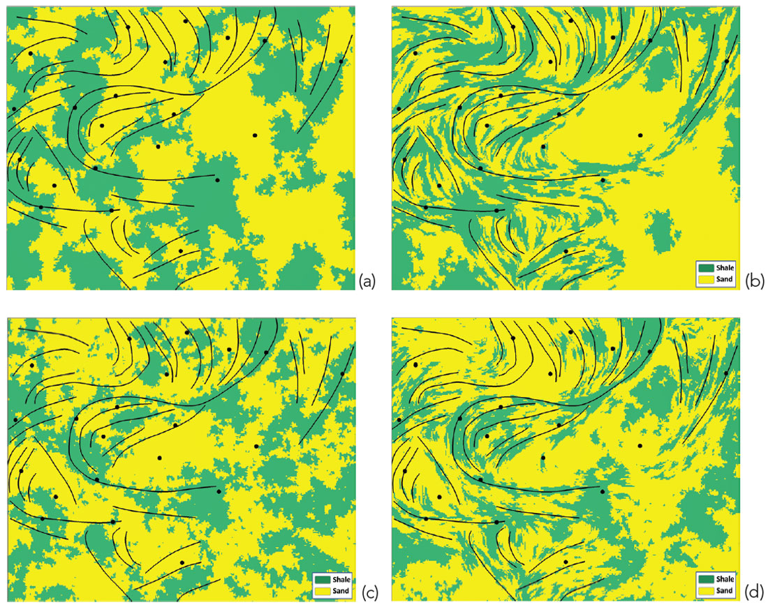
(a) single variogram model and constant lithofacies proportions;
(b) locally varying variogram model (azimuth and ranges) derived from the geomorphologic interpretation (black lines) and constant lithofacies proportions;
(c) single variogram model and locally varying lithofacies proportions derived from seismic inversion;
(d) locally varying variogram model and locally varying lithofacies proportions.
Combining geomorphologic trends, to locally influence the variograms, with lithofacies probabilities derived from seismic inversion produces more geologically realistic results. In the example of Figure 10, the mud filled abandoned channels are clearly differentiated from the sandy point bars. Channel deposits are therefore simulated with a greater geological realism with the use of local geostatistics.
Conclusions
Integrating advanced geophysical interpretation – such as seismic inversions, seismic stratigraphy and geomorphologic interpretations – into earth models helps to create more geologically realistic results.
The term “geologically realistic”, on the surface, has little place in an article whose title includes the word “quantitative”. What is meant by “realistic” in this case is a final model that has the same or better correlation to geological and engineering data, that honors the geological shape or stratigraphic elements observed in the seismic data, and that produces map view representations that pass the experienced practitioner’s “sniff test” in that they look like real geology.
Staying involved is the key to ensure the earth models and resulting flow simulations capture the geophysical interpretation and its uncertainty.

Acknowledgements
The authors would like to thank Emmanuel Gringarten, Stanislas Jayr, John Boyd, Stan Lavender, Andrew Bonvicini, Thomas Jerome and Aurelien Pierre for their comments and feedback.
A special thanks to Franck Delbecq for the many technical discussions on the subject of inversion and earth modeling over the last few years and for inviting us to write this paper in this special section of the RECORDER.
The authors would also like to thank the companies who gave permission to show pictures to illustrate this paper, including Surmont Energy Ltd., Bounty Developments Ltd. and MEG Energy.


Join the Conversation
Interested in starting, or contributing to a conversation about an article or issue of the RECORDER? Join our CSEG LinkedIn Group.
Share This Article