Quantitative Interpretation Part II: Case studies

Summary

Quantitative interpretation is the numeric estimate of the earth property of interest from geophysical data. We believe that quantitative methods are crucial to our ability to add value in the oil and gas industry. We also believe that the cultural shift necessary to fully employ quantitative methods has already begun. In part I of this work, we described the key elements of quantitative interpretation. Part II illustrates three examples of quantitative interpretation. In each of these examples, we show the value of the method in an economic argument.

The first case study is an extension of previously published work on the Viking of West central Alberta. We show the results of post application of technology and post publishing drilling on this play. These results support the value of interpolation, AVO, and the use of seismic in general. The value of these elements of geophysical effort is defined with an economic model. The second case study is concerned with steering horizontal wells in a Devonian oil play within Saskatchewan and Manitoba. We demonstrate objectively a significant increase in our ability to keep the horizontal wells within the reservoir. Steering accuracy is equated to economic value through another simple model. The third case study is another extension of previously published work; this time on the fractured Nordegg of West central Alberta. In previous work, we showed that we could predict natural fractures statistically using azimuthal methods and curvature. In this case study, we show quantitatively the relationship between the fracture density, porosity, and production rates.

Case study I: Viking economics

Introduction

Quantifying the value of seismic is rarely done, perhaps because there is a general agreement that it has value, and actually determining that value is difficult. Gray (2011) compiled numerous quantitative descriptions of the economic value of seismic, including value from 4D seismic and recovery efficiency, and general 3D seismic value. We demonstrate the value of not just the 3D seismic, but a particular processing and interpretation workflow on the Viking of West Central Alberta. Hunt et al. (2008, 2010) described the Viking project, the 3D seismic data set, the processing and interpretive workflow in detail. They showed that simple AVO attributes such as the compressional reflectivity (Rp) divided by the shear reflectivity (Rs) were useful in estimating the Phi-h of the gas-charged Viking zone. Further, they demonstrated that the AVO estimates were improved if 5D interpolation (Trad, 2009) was used prior to imaging and AVO analysis. Numerous vertical wells were used in the analysis. Seismic to well Phi-h ties were carried out by treating the Phi-h values as tops which were tied to grids of the various seismic attributes.

Numerous wells have been drilled since these studies were carried out, which allows us to determine the value of the work. We will do this by examining the accuracy of our Phih predictions against the old method (which was simply using stack amplitudes), and by examining the economic impact of the new wells. We are also afforded the opportunity of demonstrating other elements of the quantitative interpretation method, such as finding optimal attributes.

Earth properties of interest and theoretical relationships

The Viking is a tight, gas-charged sandstone. The reservoir element of the Viking may be erosionally absent, and is never thicker than one-tenth of a wavelength. It is peak on stacked compressional data, and exhibits Type II AVO characteristics (Rutherford and Williams, 1989). Based on this model response, we expect Rp versus Rs property ratios to be illustrative of reservoir quality (Castagna and Smith, 1994). Other AVO properties such as Goodway et al.’s (1997) lame parameters should also be appropriate for identifying areas of high Phi-h. These AVO methods are theoretically expected to be superior to simply using stack amplitudes for mapping Phi-h.

Processing

Hunt et al. (2008) showed that interpolation of this coarsely sampled land 3D survey was critical prior to imaging and AVO attribute estimation.

Control data

Our study area has 69 vertical or mildly deviated wells that penetrate the Viking. 23 new wells were drilled using the Hunt et al. (2008) method since the study was originally performed, of which 19 targeted the Viking specifically. We also know which of the legacy wells were drilled to specifically target the Viking, and which were drilled either without seismic or without regard for the Viking target. A few other wells were drilled subsequent to this study but were proposed by partners who did not use the new AVO method. These wells are considered “old” wells targeting the Viking. In every case, we have estimated the Viking Phi-h using multi-mineral petrophysical inversion.

Results with the best attributes

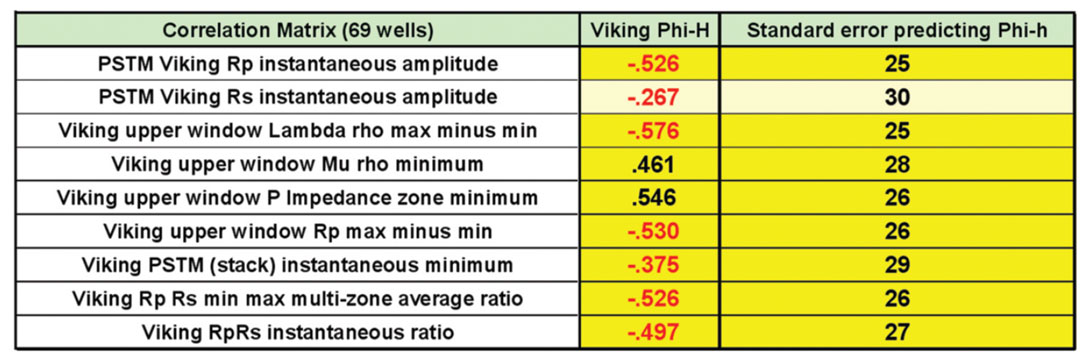
Even though we are reasonably certain that AVO properties should be better predictors of Viking Phi-h than stack amplitudes, we cannot be certain exactly what the best attribute extraction technique should be. This is the problem that concerned Schultz et al. (1994). It is very straight-forward to use the quantitative method to test a variety of attributes from the chosen properties and find out which extraction technique is optimal. Table I summarizes a subset of the attributes we tested. We evaluated this using analysis windows that started above the Viking horizon pick as well as using the amplitudes picked right at the horizon itself (which we termed “instantaneous”). This effort illustrated a minor dependence on windowing, and a stronger dependence on property. The Lambda rho property was the best single data type, followed by P impedance and Rp. This work suggests that the studies carried out by Hunt et al. (2008, 2010) might have showed an even better, albeit minor, improvement if the lambda rho property had been used instead of the Rp/Rs ratio.

Scatter plots

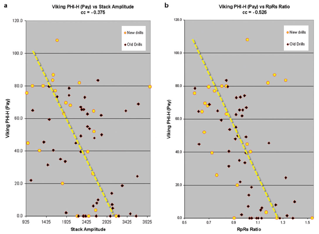
Table I showed that the AVO properties (with the exception of Rs) all yielded improvements over the stack amplitudes for predicting Phi-h. Figure 1 illustrates two of the scatter plots that accompanied the correlation work. Figure 1 (a) shows phi-h versus stack amplitudes, while Figure 1 (b) shows phi-h versus the Rp/Rs ratio. We retained the Rp/Rs ratio for the sake of consistency with the previously published work. It is clear that the stack amplitude data plot has significantly more scatter than the Rp/Rs data plot. The slope and intercept of the regression lines define transformations that allow us to create seismic estimates of Phi-h.

Results: seismic map estimates of Phi-h and identifying areas of uncertainty

One of the uses of quantitative methods is the identification of problem areas, which show up as outliers in our scatter plots. We examined the outliers in Figure 1 (b) to see if they had common characteristics. There are 4 new well outlier points in the upper right corner of Figure 1 (b); we identified those points, and found that 3 of them sat within an area previously identified as being in a strike-slip shear zone. We had previously wondered if this area would have imaging difficulties. Figure 2 illustrates critical maps of the Viking play. The end result of the quantitative method is shown as a Rp/Rs predicted Phi-h map in Figure 2 (a). The strikeslip corridor is shown by dashed yellow lines. Elements of the structure are illustrated in Figure 2 (b), which is a map of the long wavelength most positive curvature. The Phi-h values associated with each well are posted above the well symbols. AVO analysis is very sensitive to noise (Li and Downton, 2007), so it is reasonable to test the effect of culling the 4 wells within this corridor.

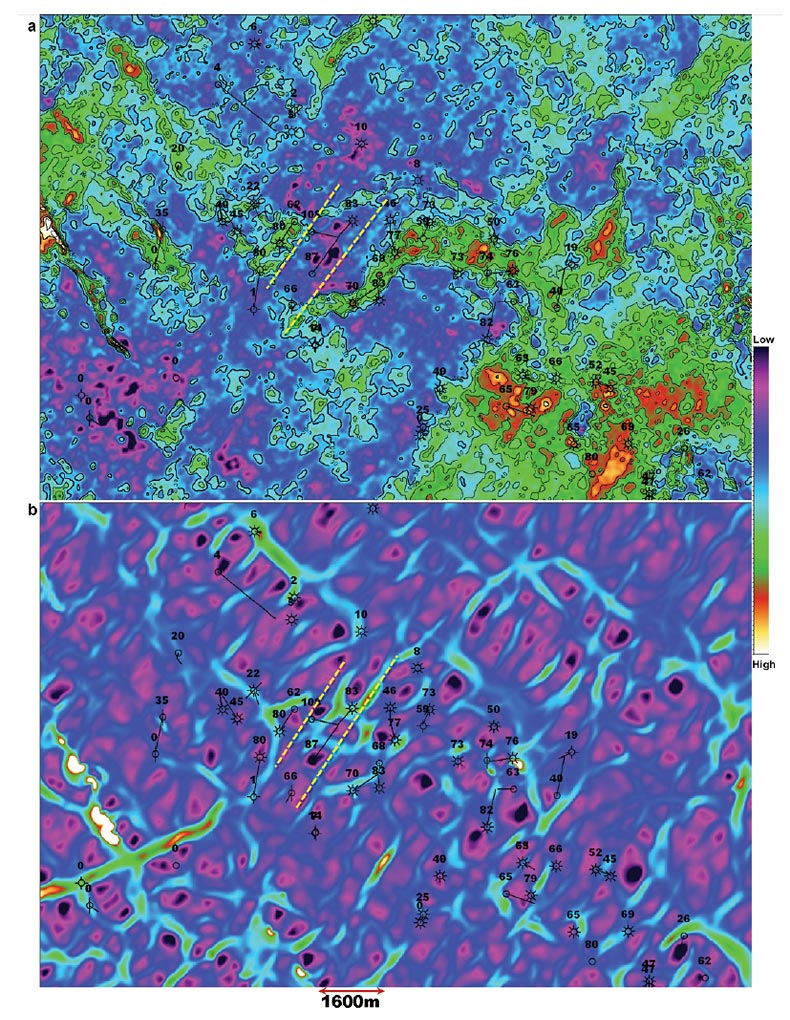
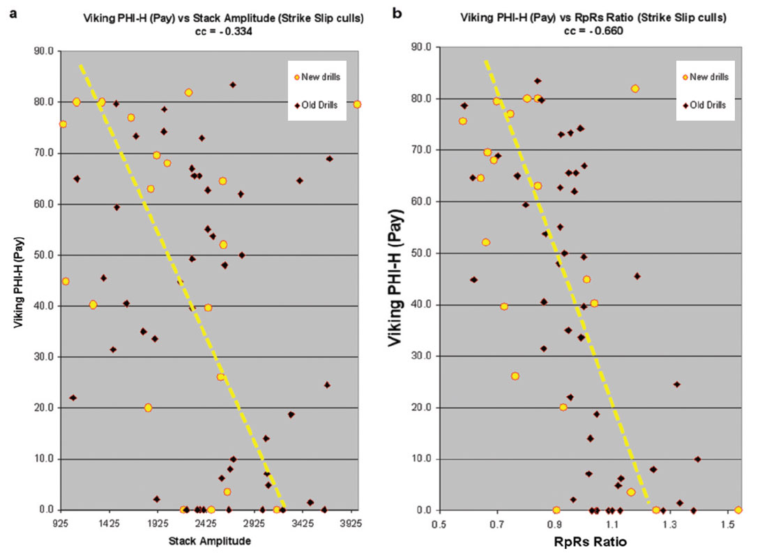
Figure 3 illustrates the effect of culling the 4 wells in the strike-slip corridor. Figure 3 (a) is the scatter plot where the stack amplitudes are correlated with the Phi-h values, while Figure 3 (b) is the same comparison for the Rp/Rs ratio. The correlation coefficient for the stack data has not improved from this culling effort, while the correlation coefficient for the Rp/Rs ratio improved significantly to -0.660. Culling may sometimes be a valid procedure; however it can create self-fulfilling conditions, and should be used carefully. This exercise likely demonstrates two possibilities:

1. That predictive accuracy varies with data quality, and therefore is not consistent everywhere on the 3D survey despite our best efforts in processing. This is a warning to carefully consider data quality changes away from control data.
2. AVO attributes are more sensitive to noise than the simpler stack amplitudes.

Value of the results

Placing a value on the increased accuracy in predicting Phi-h is not simple. Given that these methods were put forward several years ago (Hunt et al., 2008), and we have a significant body of wells drilled with the new method, production estimates can be used to estimate the value of the method. To do this, we must class all the wells in the area in the following ways:

1. Wells drilled without the use of seismic at all or without the Viking as a seismic target
2. Wells drilled using old seismic methods (post stack amplitude)
3. Wells drilled using the new seismic methods (interpolation, migration, and AVO)

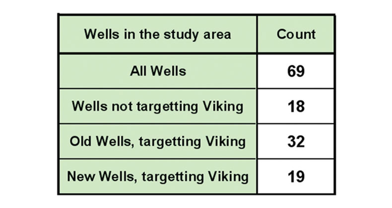
In consideration of this classification scheme, our area of analysis was enlarged. We could now consider wells outside of the area where the full AVO comparison was performed. We could also consider wells that we did not operate, or locate, but still participated in for business reasons of our own. By including a set of wells wherein the Viking was never a target, or seismic was never used, we allow two questions to be asked: what is the value of seismic, and what is the value of using seismic with this improved method. The wells in the new larger study area numbered 69, and were broken into the classes by the vice president of exploration of Fairborne Energy, at our request and without his knowledge of what we wanted to do with the information. We did this to minimize potential bias in the analysis. Table II below, describes the number of wells in each class.

The method of determining value from our seismic techniques is less direct than we would like due to the fact that most of the wells in the area have been comingled. That is, the production from the Viking zone has been combined with the production from other zones in most of the wells. No simple Viking economics, estimated ultimate recovery (EUR), or production curves can be produced for those wells. Value can still be assigned, despite this issue. Production rate and EUR can be related statistically to Phi-h in a general way using the subset of wells from the area that only produce from the Viking. A relationship between porous rock volume and economics makes physical and intuitive sense. Figure 4 below illustrates the production aspects of the phi-h economic model. Figure 4(a) shows the Viking EUR to Phi-h relationship. Although there is scatter in this chart, it is clear that higher values of Phi-h generally yield higher values of EUR. Therefore, higher Phi-h is a positive economic indicator from a reserves perspective. Economics can be calculated for Viking wells in the area given an estimate of EUR and a production curve.

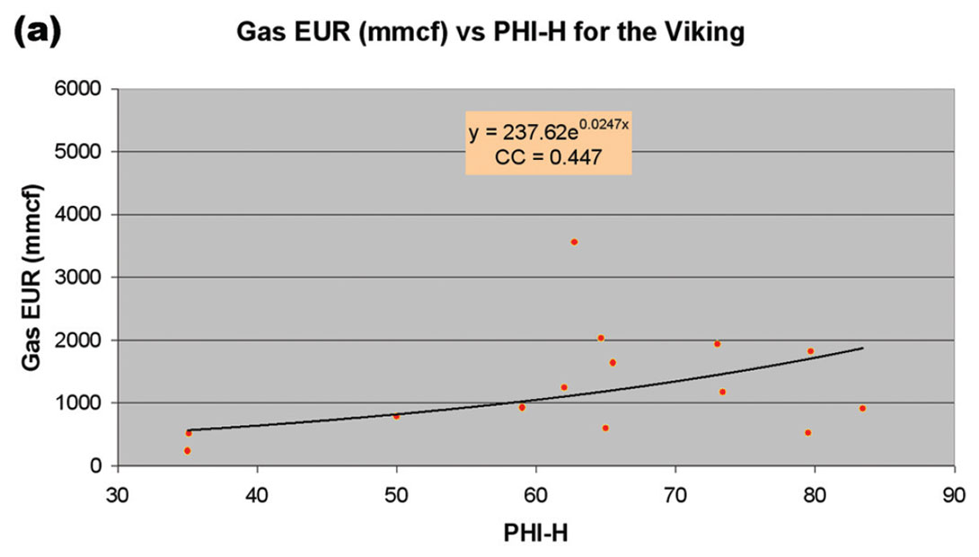
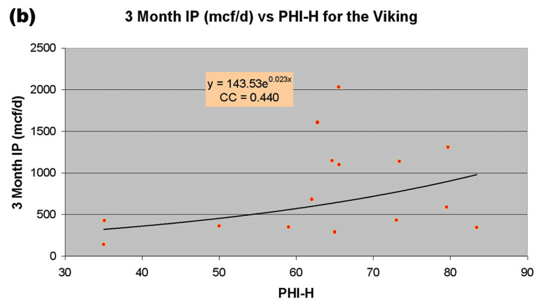
We must also consider the production curve. Three-month initial production (IP) can also be modeled with the available wells. Figure 4(b) illustrates the relationship between Phi-h and Viking three-month IP. There is again a positive correlation between these variables, indicating that Phi-h is a positive economic indicator. The scatter is similar to that of Figure 4 (a), but again the trend is physically correct.

Since Phi-h can be related to both production rate and EUR, an estimate of the economic value of any well can be statistically estimated from its Phi-h. This allows us to use the co-mingled wells in our evaluation of economic impact. We create the value estimate by averaging the Phi-h values for each of the classes of wells from Table II. We then use those Phi-h values to estimate net present values for each class. The net present values are calculated based on several factors, some of which are constant, and some of which vary:

• Constant time discount factor
• Same price deck
• Constant capital costs
• Constant rate and EUR from secondary zones, taken as an area average
• Variable rate and EUR for the Viking based on the Phi-h for each class and the modeled Phi-h and rate and EUR relationships.

Table III below summarizes these results. The new interpolation plus AVO class of wells have a significantly higher Phi-h, and net present value. The economic indicators have been shown for two different price decks.

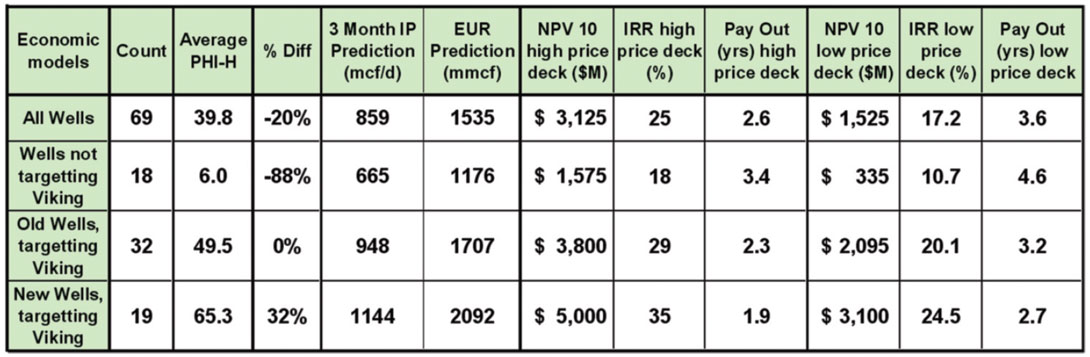
The wells drilled with the new seismic method have on average over 30% higher Phi-h values than wells drilled using the old seismic method, and a much larger relative improvement over wells drilled without seismic input. The estimated effect of using the old versus the new methods on net present value is enormous: at about a million dollars per well. The net present value estimates also address the value difference between not using seismic or geologic inference (class II is close to a drill at random selection of wells) in this area. This method of evaluation is imperfect for many reasons, including the indirect value calculation, which is unavoidable due to the co-mingled production problem. The inclusion of average secondary zones and their contributions to the flow rates, EUR, and economic value was necessary, and serves to illustrate that the secondary zones in this area are a significant factor. None of these complications and shortcomings void our results, though, since the model method is physically reasonable and even intuitively obvious. It may seem less clear that the seismic method is the only reason for the improved Phi-h in the newer wells. Certainly improved geologic insight as the prospective trends are developed must also be a factor. And yet this potential criticism of our method does not stand up either, since there have been recent wells drilled using the old seismic method and the newest geologic insight in the class II well population, and these wells have had lower average Phi-h values than the wells drilled with the new method. In fact, our newer work has resisted the common drilling trend where the best wells are drilled early in the field’s development; we are drilling our best wells now with these quantitative methods.

Case study II: steering horizontal wells

Horizontal drilling for Devonian oil targets is a major element of exploration and development investment in South-East Saskatchewan and Manitoba. Many of the target reservoirs are relatively thin and structured, which presents challenges to steering these wells. Prior to this work, we did not use seismic to steer horizontal wells on this play. Although we were able to keep our horizontal wells in the reservoir most of the time, there were cases where we failed to steer the wells with confidence. We show the value of seismic to improve horizontal well steering accuracy and productivity for this target.

Earth properties of interest and theoretical relationships

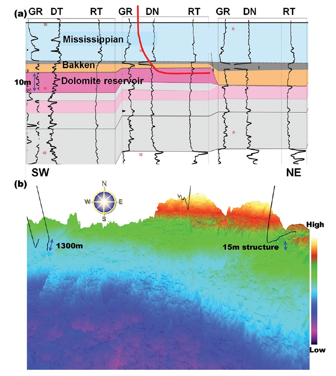
Our target is a Devonian-aged dolomite reservoir, underlying the low impedance Bakken shale. The reservoir varies from 3m to 10m thick in the study area, and is structured. Figure 5 illustrates the stratigraphy at the reservoir level, and the structure in the local area. The sample horizontal well paths depicted in Figure 5(b) demonstrate structural features greater than the thickness of the reservoir.

Processing

We were required to reprocess the 3D seismic data to improve the resolution in order to carry out the time to depth conversion. Accurate time to depth conversion requires several practical conditions be met:

1. All major velocity changes are pick-able on the seismic.
2. The target is also pick-able on the seismic. This implies that the pick is stable and represents the true reservoir level.
3. There must be an abundance of well control to define the velocity field.

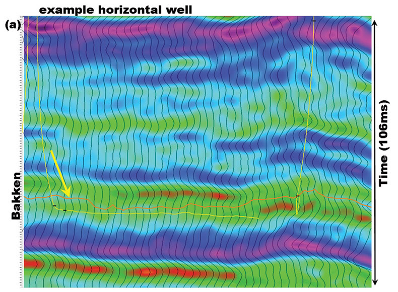
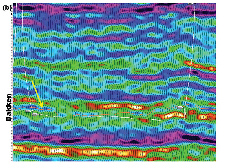
The original 3D seismic data was not of sufficient quality to pick the Bakken shale, which we use to estimate the depth of the reservoir. This is a failure of requirement #2 for time to depth estimation. A line from the original processing is illustrated in Figure 6(a), and shows the Bakken shale is not resolved. Simple post-stack spectral enhancement failed to sufficiently improve the resolution of the data. Figure 6(b) shows the same line with spectral balancing added. The resolution is increased significantly, but the data is still not resolved well enough, and is too noisy for practical use. It is not yet possible to pick the Bakken shale with confidence.

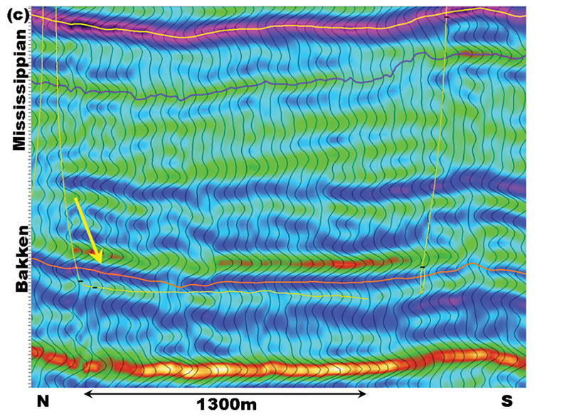
We reprocessed the data to increase the resolution and suppress the noise. Hunt et al. (2005) showed that reprocessing using multiple nested noise attenuation and deconvolution steps in conjunction with pre-stack interpolation could be effective in increasing the resolution of even tightly shot land 3D seismic surveys. The role of interpolation for this purpose was further discussed by Hunt (2009). We employed these methods in our reprocessing, and were successful in improving the effective resolution of the data sufficiently to pick the Bakken shale. Figure 6(c) shows the sample line after this reprocessing. The data is much higher resolution, and has a high signal to noise level. The Bakken shale is apparent, and pick-able. This work enabled accurate time to depth estimation to take place.

Control data

The study area had over 60 vertical wells in addition to 25 horizontal wells that we had drilled prior to this work. All of this well control was used in the time to depth estimation. The 25 existing horizontal wells form our statistical measure of the old method of steering, which made only minimal use of seismic.

Results with the best attributes

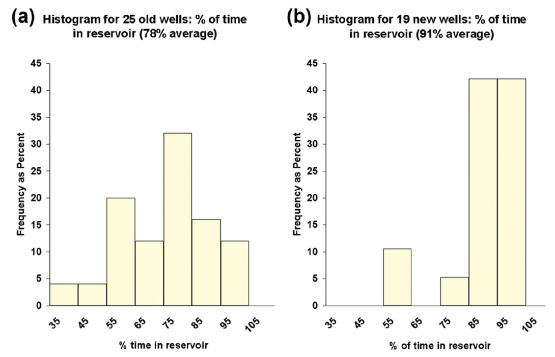
We have drilled 19 new horizontal wells using the reprocessed data and the time to depth estimation. Figure 7 illustrates the improvement in steering accuracy. We coded each well by lithology based on the well-site data, and noted what percentage of the time each well was steered within the target reservoir. These percentages form the histograms of Figure 7. Figure 7(a) shows that the original 25 wells were steered within the reservoir 78% of the time on average. Figure 7(b) shows that the 19 wells that we drilled after reprocessing and time depth estimation were steered within the reservoir 91% of the time. This significant improvement is entirely due to the increased use of seismic.

Value of the results

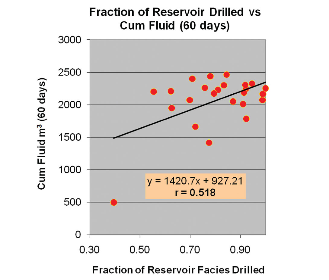
Determining the value of the improved steering is not straightforward, and requires performance modeling. The reason for this is that we cannot simply compare well rates between old and new wells due to significant changes in completions and equipping that took place at the same time as our seismic effort. Our new wells vastly outperform our old wells for a variety of reasons. In order to estimate the value of steering, we make reference to the production statistics of the original 25 wells. Figure 8 is a cross plot of percentage time in reservoir versus the 60 day cumulative fluid produced. The cross plot has scatter, but has a positive correlation, which is physically expected. This means that wells drilled within the target were generally more productive than wells that were less successfully steered. Although these first 25 wells were completed and produced in a similar manner, even small changes in these practices are responsible for some of the scatter seen in the cross plot.

The regression fit to Figure 8 can be used to determine the average 60 day cumulative fluid production for the first 25 wells. This same fit can be used to estimate the cumulative production for the 19 wells that were steered with seismic if completion and production practices had been kept constant. These cumulative numbers can be used to calculate average 60 day initial production rates. The difference in production thus arising from 91% steering accuracy versus 78% steering accuracy is over 19 barrels per day per well. The value of this depends on netback and water cuts. If we apply our average area net backs and water cuts to this number, we expect that the steering improvement is worth more than $400 per well per day for this area. For the 19 wells drilled to date, this is greater than $7600 per day. Our new wells actually perform better than this.

Case study III: fractures and production

The Nordegg Formation in the West Central Alberta was described by Hunt et al. (2010a) as a gas-charged, tight, fractured sandstone reservoir. This work showed that surface seismic attributes such as long wavelength most positive curvature (curvature) and amplitude versus offset and azimuth (AVAz) had a statistical correlation to fracture density as validated with image log data from two horizontal wells and microseismic data. This case study is an extension of Hunt et al.’s (2010a) work, and shows that these seismic attributes are also correlated to production and fracture treatment behaviour.

Earth property of interest and theoretical relationships

Nelson’s (2001) extensive work on fractured reservoirs recognized that both the matrix and fracture porosities and permeability should be considered for a wide variety of reservoirs. Our image log data estimates that the fracture contribution to porosity is not significant, leaving the fractures’ effect on overall permeability as the key fracture-related question for the Nordegg. In the absence of changes in reservoir damage, and under similar pressures, permeability characteristics will dominate the early flow capability of similarly completed wells. But do fractures help or hinder production? This question cannot be answered generally, since each fracture system is unique (Nelson, 2001). Dunphy and Campagna (2011) described further how the answer to this question is subject to many unique parameters individual to each formation, facies, play, area, and sometimes even to each spacing unit. This increases the need for quantitative measures. The simplest representation of the performance of a reservoir with a single fracture system was described by Nelson (2001):

Q = C ( k_matrix + k_fractureCos α ) P   which becomes:
Q = C ( k_matrix + (e³ /12) D_f Cos α ) P

where Q is the rate, C is a term that includes area and viscosity terms, P is a term related to the pressure draw down, k_matrix is the matrix permeability, k_fracture is the fracture system permeability, and α is the angle between the pressure gradient and the fracture plane. The Fracture permeability is seen as a being dependent on the fracture aperture, e, and the fracture density, D_f. The fractures are treated as vertical plates and are assumed to behave independently with respect to the matrix permeability. This equation can also be expanded to treat multiple fracture sets. A key implication to this formula is the linear relationship between fracture density and production rate at a given angle to the fracture plane.

A complication to this simple model is the fact that we will fracture- stimulate the Nordegg. Our image log data indicates that most of our fractures are partially mineralized. The question then becomes: are those fractures likely to reopen under fracture stimulation without adversely affecting the stimulation operation itself? Another question is: will the fractures re-open somewhat easier than the surrounding un-fractured matrix? If the fractures can be re-opened easier than the rest of the matrix, but not so easily that they actually prevent fracture stimulation to occur, we might expect to see two things:

1. Higher production over intervals with greater fracture density
2. Lower fracture gradients over intervals with greater fracture density.

Control Data

There is extensive 3D surface seismic coverage in the area which enabled the identification and mapping of the major structural features of the Nordegg. Three wells (Well A, B, and C) were drilled into several of the interpreted structural archetypes present in the area. Figure 9 illustrates these structural archetypes and the relative positions of the wells.

Well A was drilled along the strike of an anticlinal feature, Well B was drilled into a major strike slip feature, while Well C was drilled in a relatively unstructured setting. Image logging was performed for Wells A and B, and included fracture density measurements. A full suite of other wireline logs were also run over Wells A, B, and C, including Gamma Ray, resistivity, bulk density, and full waveform sonic data. These logs can be used to estimate porosity. After the wells were completed, flow tested, and put on production, production logging was run for each stimulation zone in the three wells.

Processing

This data was processed using noise attenuation, resolttuion enhancement, and interpolation prior to azimuthally sectored migration as described by Hunt et al. (2010a, 2010b). Pre-stack interpolation was important for this data set, and its effect on AVAz was shown by Downton et al. (2010).

Method

The three horizontal wells each had eight completion zones. The completion parameters for each zone were planned to be identical, and although the actual completions were imperfect, the stimulations were very similarly executed in most of the zones. Each completion zone is isolated by packers. Production logging data provided flow estimates for each of the completion zones in each well, giving a total of 24 data points. The data was presented as a percentage of total flow. The percentage flow rates were normalized by the absolute open flow (AOF) estimated for each well so that the flow data could be used for all the wells together. The fracture gradient was also calculated from the completion operation for each interval, and gives another 24 data points to validate the seismic attributes with. There are advantages and disadvantages to the use of the production test data and the fracture gradient data as validators. Both data types are subject to some interpretation. Production data has obvious, clear- connections to economic value, but fracture gradient data may be less subject to operational complexities and error.

The simplest method of comparing log and seismic attributes to production and completion data was to average the attribute values over each completion zone, to produce comparable data points. These sets of data were cross plotted and the strength of their correlations could be determined. This was our primary method of analysis for each of the candidate attributes, and it was first applied to the well log data. In the case of the well log data, we averaged attributes of estimated porosity from a multimineral log analysis and fracture density from the image log. The log test was a critical first step since our dual permeability hypothesis requires the matrix porosity and the image log fracture density to correlate to production data. This initial test is required to encourage the seismic comparison to the production data. The seismic estimates of porosity were created from amplitude dimming on the Nordegg, and the curvature and AVAz estimates were directly from Hunt et al. (2010a).

Results

The various capture and averaging of log and seismic attributes was carried out as described above. Numerous regressions against the production and fracture stimulation data were then performed. Figure 10 and Figure 11 summarize the key results. Figure 10 compares the production from each completion interval against either log data or seismic attributes. The data points for each well are color coded. Figure 10(a) shows a positive correlation between log measured porosity and production, which is expected. Figure 10(b) shows a positive correlation between image log fracture density and production, which is also expected. These two results are encouraging, and suggest the seismic estimates of porosity and fracture density may also be correlated to production. Figure 10(c) shows a positive correlation between seismic estimated porosity. Figure 10(d) shows a positive correlation between AVAz anisotropic gradient and production. All of these correlation coefficients were of similar value, and they all showed some clustering for each well. The correlations for each well individually are significantly poorer, which is apparent in the scatter plots. When the three wells are used together, the apparent correlations are quite good. We speculate that the reasons the three wells behave differently is because they sample three different structural regimes in the data, as shown in Figure 9. Well A has the best overall production performance, had the most fractures in image logs, had the highest overall log porosity, highest curvature, and highest AVAz. Well C performed worse than well A and better than well B on a production basis. It was drilled in a flat area with little inferred fractures, and with porosity better than well B but not quite as good as well A. Well B was the worst well on a production basis, had the lowest log and seismic estimated porosities, and had the lowest AVAz values. It is difficult to be certain if porosity or the fractures are the dominant driver of production. The simplest interpretation of this data follows Nelson’s (2001) idea of a dual permeability system in which both matrix permeability and fracture density are important.

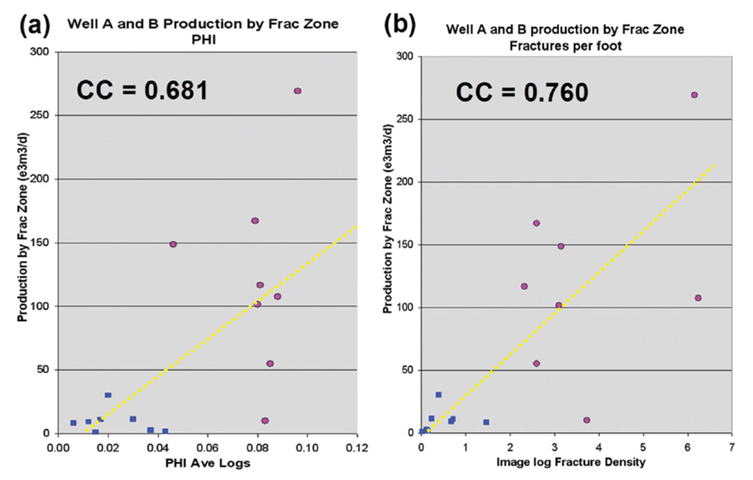
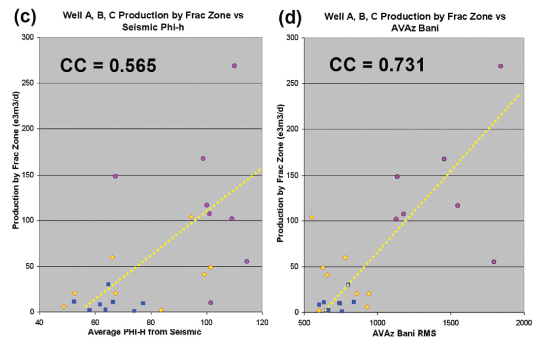
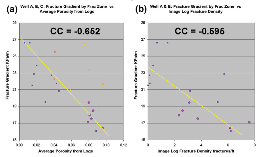
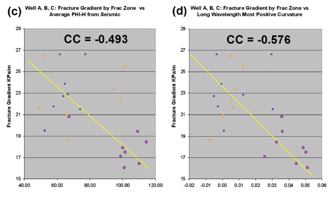
Figure 11 compares the fracture gradient from each completion interval against either log data or seismic attributes. Lower fracture gradients suggest greater ease of fracturing. Figure 11(a) shows a negative correlation between log measured porosity and fracture gradient, which is expected. Figure 11(b) shows a negative correlation between image log fracture density and fracture gradient, which is also expected. These two results are encouraging, and suggest the seismic estimates of porosity and fracture density may also be correlated to fracture gradient. Figure 11(c) shows a negative correlation between seismic estimated porosity. Figure 11(d) shows a negative correlation between curvature and fracture gradient. The same well by well clustering of data is apparent in these scatter plots. We chose to show curvature in Figure 11(d) because curvature may be related to fracture density, or in the case of well A, may indicate an area of extension and possible release of compressional stress. Such a location may fracture stimulate easier (Goodway et al., 2010). The negative correlation in Figure 11(d) between curvature and fracture gradient could be interpreted as suggesting either possibility.

Conclusions

Our three case studies demonstrated objective, measurable value from seismic to current exploration and development projects. Quantitative methods were required to measure this value. We showed that reprocessing was required to make accurate time-depth estimates possible, and to enable more accurate AVO analysis. We also showed that fractures may have a significant effect on Nordegg productivity.

These examples span the importance of geophysics operationally in steering horizontal wells, in addition to their more familiar role in the pre-planning of wells. The specific results of this work may not be general, but the value of the quantitative method itself is. Without this method, we cannot measure value, determine advantage, steer wells, find the best attribute, transform attributes to geologic properties, or try to determine what geologic features are even important. Quantitative methods encourage us to be better scientists, to commit to predictions, observe their accuracy, and to communicate with our peers in the language of the earth properties with which we are all concerned.

Acknowledgements

We would like to thank Fairborne Energy Ltd for permission to show this work, and CGGVeritas Multi-Client Canada for permission to show data licensed to them. We would also like to thank Nicholas Ayre, Emil Kothari, Alicia Veronesi, Alice Chapman, Dave Wilkinson, Dave Gray, Darren Betker, and Earl Heather for their work on this project, and Satinder Chopra for his advice.