Microseismic Moment Tensors: the Good, the Bad and the Ugly

Summary

Seismic moment tensors provide a general mathematical representation of point sources that can be used to distinguish between various microseismic source types. We use synthetic tests with borehole receiver arrays to determine the geometrical conditions necessary to estimate reliably the six independent components of a full moment tensor by leastsquares inversion. We show that the solid angle subtended by the receiver array, as viewed from the source location, plays a fundamental role in the stability of the inversion. In particular, the condition number of the generalized inverse scales linearly with the solid angle, implying that for a solid angle of zero (as is the case for a single vertical borehole) the inversion is ill-conditioned. Our numerical tests indicate that least squares moment-tensor solutions obtained under such nonideal conditions tend to be biased toward double-couple (i.e., mode II or II fracture) mechanisms. Our findings suggest that caution should be exercised in the interpretation of momenttensor solutions from microseismic field experiments. Possible strategies to alleviate this concern could be to ensure a nonzero solid-angle aperture by using multiple observation wells, or to incorporate other types of data such as a priori knowledge of fracture orientation to constrain the solutions.

Introduction

Seismic moment tensors provide an idealized mathematical representation of rupture processes within the Earth. In global seismology they have been in routine use for decades and provide valuable insight into earthquake mechanisms. They are traditionally presented as focal mechanism (a.k.a. beach ball) diagrams, which depict the amplitude radiation pattern for P-waves and reveal, at glance, the type of fault and possible orientations of the fault plane.

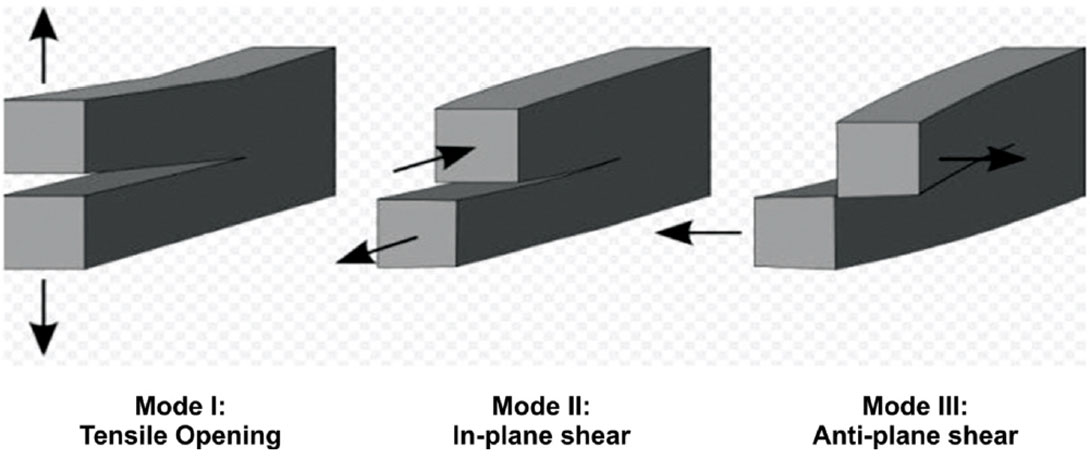
Monitoring microseismicity induced by hydraulic fracturing processes, geologic sequestration of carbon dioxide and geothermal field development has the potential to improve our understanding the fracture process and optimize reservoir production (Lumley 2001; Shoham 2001). Moment tensors can provide information about the inducing mechanisms, size and orientation of fractures and the connectivity of fracture systems (Maxwell and Urbancic 2001; Foulger et. al. 2004), and whether the fracture is opening or closing (Kirkpatrick, et al. 1996). As illustrated in Figure 1, fracture processes that cause microseismicity may include tensile opening of a fracture (mode I) or slip on a pre-existing fracture surface (modes II and III) that do not result in any net porosity change. Accurate estimation of moment tensors using microseismic data, however, remains a significant challenge due to the low signal-to-noise recording conditions and typically small-aperture acquisition geometry.

This paper considers some of the limitations of momenttensor inversion in a microseismic monitoring environment. After briefly reviewing moment-tensor theory, we use a synthetic modeling approach to assess the fundamental geometrical constraints on inversion for moment tensors. We show that the solid angle subtended by the microseismic array, viewed from the source location, is a key consideration for stability of the inversion. Building on this concept, we then consider the question of whether any bias exists for moment tensors obtained by least-squares inversion of data from a single vertical observation well.

Theory

Seismic moment tensors can be represented as a 3 3 array, normalized to unit amplitude (e.g., Lay and Wallace, 1995),

where M₀ is the seismic moment and each element Mij represents a force couple composed of opposing unit forces pointing in the i-direction, separated by an infinitesimal distance in the j-direction. Conservation of angular momentum imposes the condition that M is symmetric, reducing the number of independent moment-tensor elements to 6 in any co-ordinate system.

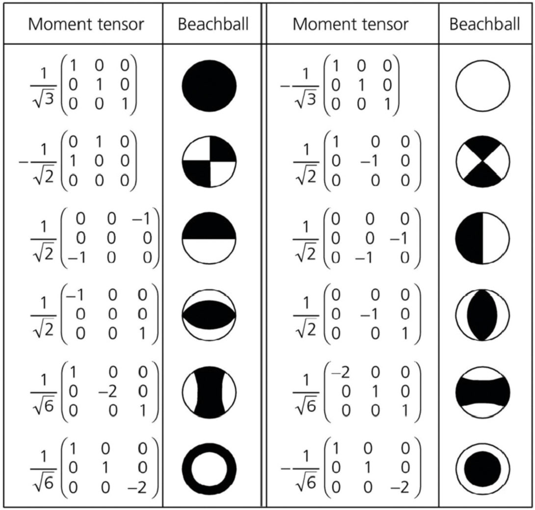
A particularly simple moment tensor is the so-called double couple, which describes the radiation pattern for slip on a fracture. A double couple can be represented using two equal, nonzero offdiagonal elements. Although most earthquakes can be well represented by double-couple mechanisms, other mechanisms are sometimes used. For example, the identity matrix corresponds to an isotropic volumetric expansion (explosion) and the compensated linear vector dipole (CLVD) has a double-strength force couple in the direction of one eigenvector and unit-strength force couples in the directions of the other two (Lay and Wallace, 1995). The latter has been used to represent tensile events that occur in hydraulic fracturing due to nucleation and propagation of the fracture into a competent rockmass (Nolen-Hoeksema and Ruff, 2001). Figure 2 illustrates some selected moment tensors and their associated focal mechanisms (beach ball diagrams) for various seismic sources.

For a homogeneous region around a source located at the origin, the ith component of particle motion arising from the radiated Pwave can be written as (Lay and Wallace, 1995)

where ρ and α are density and P-wave velocity, γ_i is a direction cosine of the receiver position vector, r is the source-receiver offset, the dot notion denotes time derivative and the summation convention for repeated indices is used. Similarly, the radiated Swave may be written as

where β is shear-wave velocity and δ_ij is the Kronecker delta.

The relationship between the data and model components can be written in matrix form,

where d = (a₁^P, a₂^P, a₃^P ,a₁^S ,a₂^S ,a₃^S )^T defines the observed amplitudes of the P- and S-wave direct arrivals and m = (M₁₁ , M₂₂ , M₃₃ , M₁₂ , M₁₃ , M₂₃)^T defines the independent components of the seismic moment tensor. For a single receiver, the 6 6 matrix A can be easily surmised from equations (2) and (3). For n receivers, the 6n 6 system can be formed by appending additional rows, as required, onto d and A. A least-squares solution to this over-determined system can be obtained using the generalized inverse,

In most of the examples below, the generalized inverse is illconditioned. In such cases, the number of resolvable components of m is assumed to be equal to the number (N) of significant eigenvalues of A^TA. Significant eigenvalues are defined here as those with absolute value greater than one ten thousandth of the absolute value of the largest eigenvalue. The best resolved component of m is taken as the largest component of the eigenvector that corresponds to the largest eigenvalue.

Results

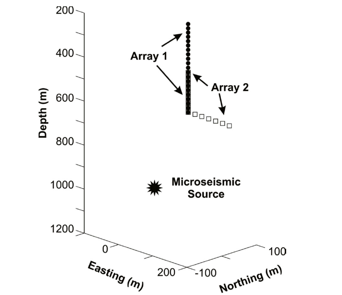
As illustrated in Figure 3, several scenarios are considered here to investigate the resolution of m using realistic borehole receiver arrays. The source is located at x = y = 0 and a depth of 1000 m.

Array 1 represents a vertical set of receivers between 200-700 m depth, located 100 m north of the source. Array 2 represents is located between 500-700 m depth and includes a 100 m borehole deviation to the east. Receivers are shown every 20 m in Figure 3, but numerical tests show that 2-3 receivers at the corner points give equivalent results (i.e., sparse observations are sufficient for moment-tensor inversion).

Different seismic moment tensors predict different relative amplitudes and polarities of P- and S-wave arrivals. This concept is illustrated in Figure 4, which shows synthetic seismograms for two different moment tensors, a double couple and a CLVD source. It is these differences in amplitude and polarity that render it possible to distinguish different seismic sources.

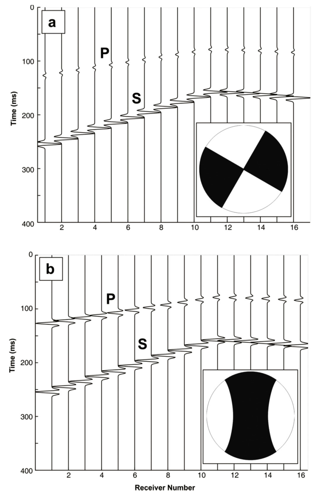
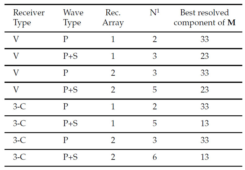
Table 1 summarizes a series of tests conducted using both arrays in conjunction with either vertical and three-component (3-C) receivers. In addition, analyses of P-wave only, or both P- and Swaves are considered. The results of these tests indicate that the full moment tensor (6 independent components) can only be obtained using 3-C receivers using array 2, coupled with the analysis of both P-waves and S-waves. In general, numerical tests indicate that a necessary condition for the moment tensor to be fully resolved is that the receiver array subtends a solid angle Ω > 0, viewed from the source. The solid angle is given by

representing the surface area subtended on the unit sphere, in the same way a planar angle equals the length of an arc of unit circle. It has a range from 0 to 4π steradians.

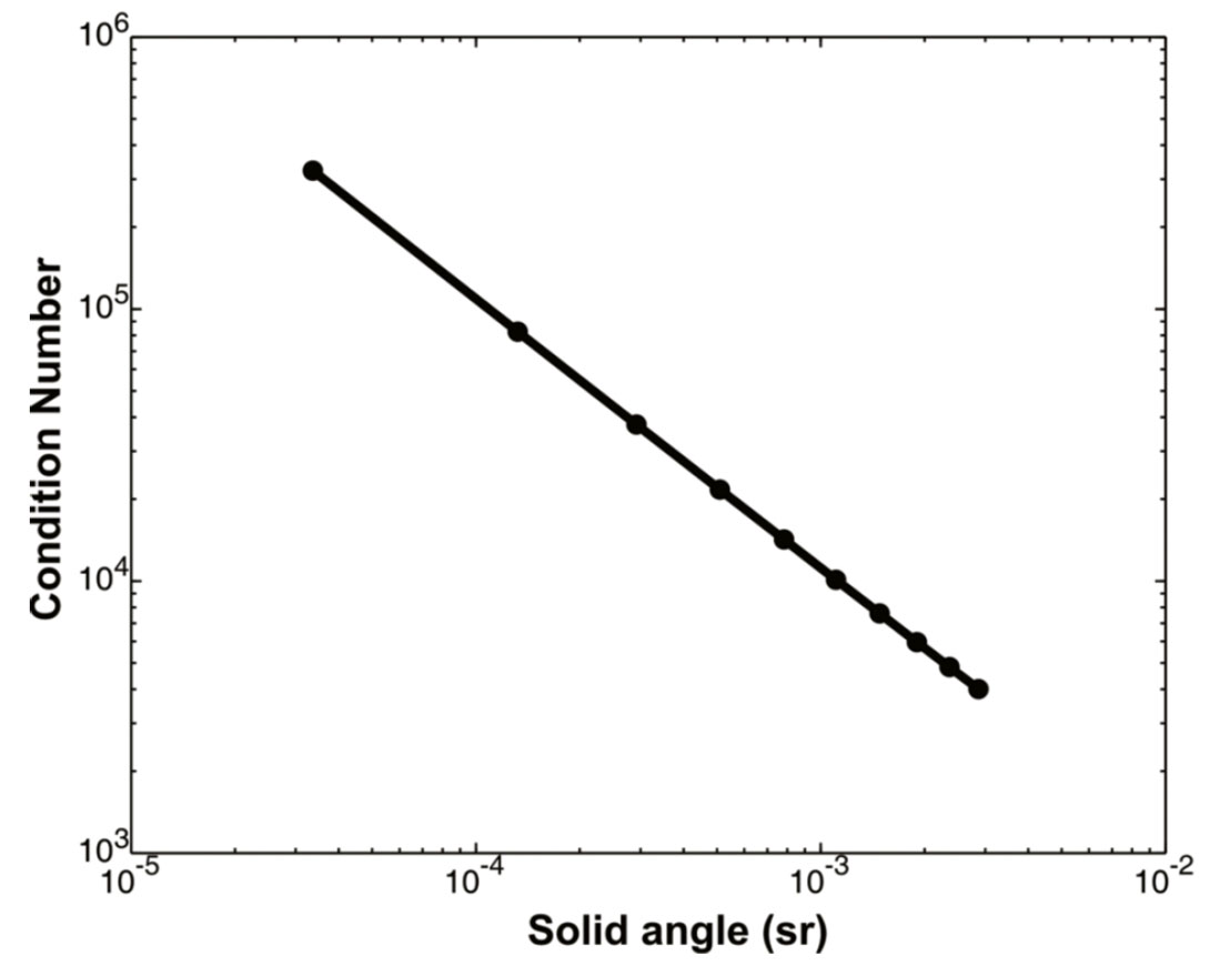
As shown in Figure 5, for cases where m can be fully resolved (i.e., 3-C receivers, both P and S analyzed, Ω > 0), synthetic tests show that the condition number of A^TA is linearly related to Ω^-1. Thus, the geometry of the receiver array should be designed to maximize the field of view, as seen from the source. Vertical arrays of geophones do not accomplish this, since the solid angle subtended by the array is zero. In general, Ω can be increased by using a deviated borehole and/or multiple boreholes, as well as by placing the receivers as close as possible to the source.

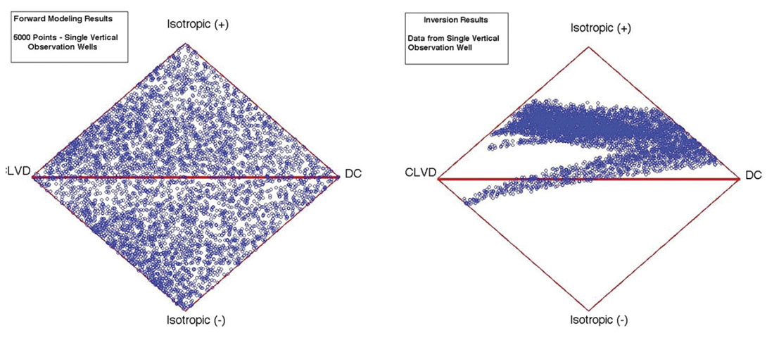
Although the moment-tensor inverse problem is ill-conditioned for the common scenario of a single vertical observation well, a least-squares solution can still be obtained by imposing an additional condition such as minimum deviation from an initial guess. We are therefore motivated to ask whether any inversion bias is likely to arise in this case. To investigate this, we have conducted a synthetic seismogram study using an assumed borehole acquisition geometry modeled on an actual field program, similar to array 1 (above). For this set of tests, we assumed a microseismic source at depth of 2 km and a receiver array in a vertical well composed of 12 geophones with 11.5 m spacing. We generated synthetic seismograms for 5000 source mechanisms with random combinations of isotropic (ISO), CLVD and double-couple (DC) components (Fig. 2). We then used the synthetic waveforms to invert for the moment tensors and decompose them into the ISO, CLVD and DC components. Without preconditioining, the inverse problem is ill-posed; consequently the leastsquares inverted solutions differ from the input mechanism.

The results of this synthetic study are illustrated on the ternary diagrams in Fig. 6. In general, we find that the distribution of inverted focal mechanisms maps to a sub-region of the parameter space that is close to the double-couple (DC) end member. This result is consistent with the previous discussion showing that a necessary condition for the moment tensor to be fully resolved is that the receiver array subtends a nonzero solid angle viewed from the source. This condition is not met in the case of a single observation well.

Conclusions

Our findings suggest that caution should be exercised in the interpretation of moment-tensor solutions from microseismic field experiments. Least squares solutions that are based only on P- and S-wave amplitudes tend to be biased toward doublecouple mechanisms. Possible strategies to alleviate this concern could be to ensure a nonzero solid-angle aperture, or to incorporate other types of data, such as a priori knowledge of fracture orientation, to constrain the solutions.

Acknowledgements

We gratefully thank the sponsors of μ-SIC (micro-Seismic Industry Consortium) for their financial support of this project. This work was also supported by a Discovery Grant from the Natural Sciences and Engineering Research Council.