Microseismic Location Uncertainty

Summary

Microseismic imaging is a common technique for mapping hydraulic fractures. Accurate imaging of the source location of the microseisms is critical for accurate fracture mapping. In this paper, two simple synthetic examples are presented which demonstrate the mislocation that could result from data and velocity model errors. Location errors resulting from intentionally processing with inaccurate velocity models are presented to highlight an important quality control plot of arrival time differences that can be used to identify systematic apparent velocity errors in the arrival time moveout. This provides a simple velocity model quality control for interpretation by non-specialists and offers the possibility of velocity model inversion and quantification of velocity model errors for sensitivity tests. Monte Carlo simulations are also used to demonstrate random location uncertainties resulting from input data uncertainties in arrival times and raypath polarizations. The results highlight the interaction between mislocations from both input data random uncertainties and systematic velocity model errors. The errors are also shown to significantly change with geophone array geometry, and demonstrate the possibility of optimized sensor placement to improve location accuracy. For example, modeling of the Horn River Basin in NE BC, illustrates significantly improved accuracy with certain geophone locations.

Introduction

Microseismic imaging of hydraulic fracture stimulations is a common technique to determine fracture geometry and growth characteristics, and has been utilized in most formations in the WCSB. These stimulations correspond to high pressure injection of fluids, and are necessary to enhance permeability for economic oil and gas production in many reservoirs. Microearthquakes associated with either creation of new fractures or activation of pre-existing fractures are used to image the hydraulic fracture growth. Microseismic images can provide critical data for optimization of both the fracturing process and resulting production from the well.

Various aspects of the fracturing can be assessed by processing the microseismicity detected during the injection, although one of the most fundamental parameters is the hypocenter of the source location of the microearthquake. The spatial-temporal characteristics of these microseisms result in a 4D image of the fracture growth. The hypocentral location of a microseism is computed by finding the spatial position which best matches observed arrival of various phases in the recorded microearthquake seismogram. This computation requires a velocity structure for forward modelling of theoretical phase arrival times.

Construction of a velocity structure requires sufficient detail to accurately predict arrival times in order to accurately reproduce the source location. Depending on the lithologic details of the reservoir, velocity heterogeneity and anisotropy characteristics may need to be accounted for. However, routine microseismic processing often utilises minimal velocity structure information, often based mainly on sonic logs recalibrated with limited data such as a calibration shot from a known location. Typically this recalibration is a nonunique under-determined velocity inversion of the true velocity structure. As with any geophysical seismic velocity construction, the resulting velocity model will have some intrinsic uncertainty resulting in an associated location uncertainty in the microseisms.

In addition to the location uncertainty resulting for the velocity model uncertainty, another factor is uncertainties in the observed input data of arrival times and raypath polarizations. The input data uncertainties are typically a random element, but relate to non-linear random uncertainties in the event locations (ie. location precision). Monte Carlo simulation offers a convenient means of quantifying this random location error by varying the input data according to the expected uncertainty of the arrival times and directional data. The velocity model uncertainty tends to relate to a systematic mislocation (ie. location accuracy), depending on the characteristics and limitations of the assumed velocity model. In this paper, these two aspects of the location uncertainty will be demonstrated by applying a Monte Carlo technique to quantify the random errors, and also an extreme bulk shift of the velocity model will be used to demonstrate in interaction with systematic velocity related errors. The velocity model errors will be assumed for a worse case scenario to maximize the systematic location errors for demonstration purposes. The objective of the synthetic modelling studies presented here are two fold. Firstly, one example of the Barnett Shale is intended to demonstrate a processing attribute that can be used for quality control of the velocity model accuracy. Secondly, modeling based on Horn River Basin lithologies is used to demonstrate how geophone array positions can be strategically positioned to reduce possible location errors.

Barnett Shale Model

A velocity model was assumed, which is loosely based on the lithology of many shale gas plays such as the Barnett Shale of the Fort Worth Basin in Texas. The Barnett is the site of extensive microseismic imaging of hydraulic fracture complexity associated with injection in the naturally fractured shale. The shale corresponds to relatively low velocities, with relatively fast limestone units above and below. This lithologic section is typical of a number of other shale gas formations with shales contained in more competent rocks. The velocity contrasts between these formations result in significant seismic wave refractions which serve as a useful demonstration of extremes in event location errors associated with velocity errors. Figure 1 shows the assumed velocity model, with a low velocity shale unit between 8000’ and 8200’.

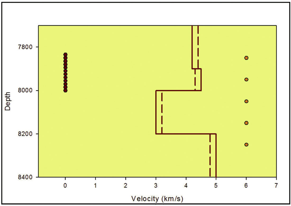
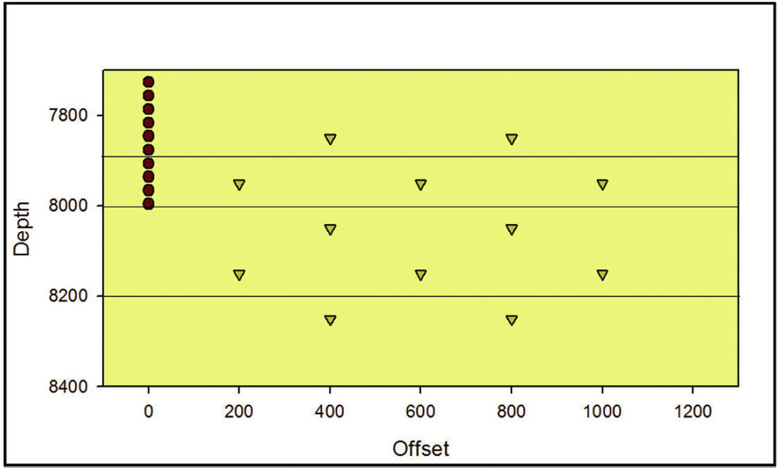
Figure 1 also shows the depth of the sensors and sources assumed for the synthetic calculations as well as an incorrect velocity model which will be referred to in subsequent analysis. Sources are distributed above, below and within the shale interval. In this example, the depth of the sensors is above the shale, which is typical of many microseismic monitoring examples where wellbore plugs are used to isolate open perforations for pressure control when existing production wells are used as an observation well. Figure 2 shows assumed source positions, which are all located in a vertical plane at various horizontal offsets from the geophones as indicated. Based on this geometry and velocity model, arrival times and directions were computed for each source and sensor. A constant Vp/Vs ratio was assumed to compute both p- and s-wave arrival times.

Synthetic event locations were first computed using assumed arrival time and directional uncertainties of 0.5 ms and 5º respectively, with the correct velocity model. For each source position, a 100 iteration Monte Carlo simulation was computed with the arrival times and direction data perturbed using a random number generator following a Gaussian sampling from the assumed data uncertainties. For each Monte Carlo iteration, a new source location was computed for that perturbed arrival data.

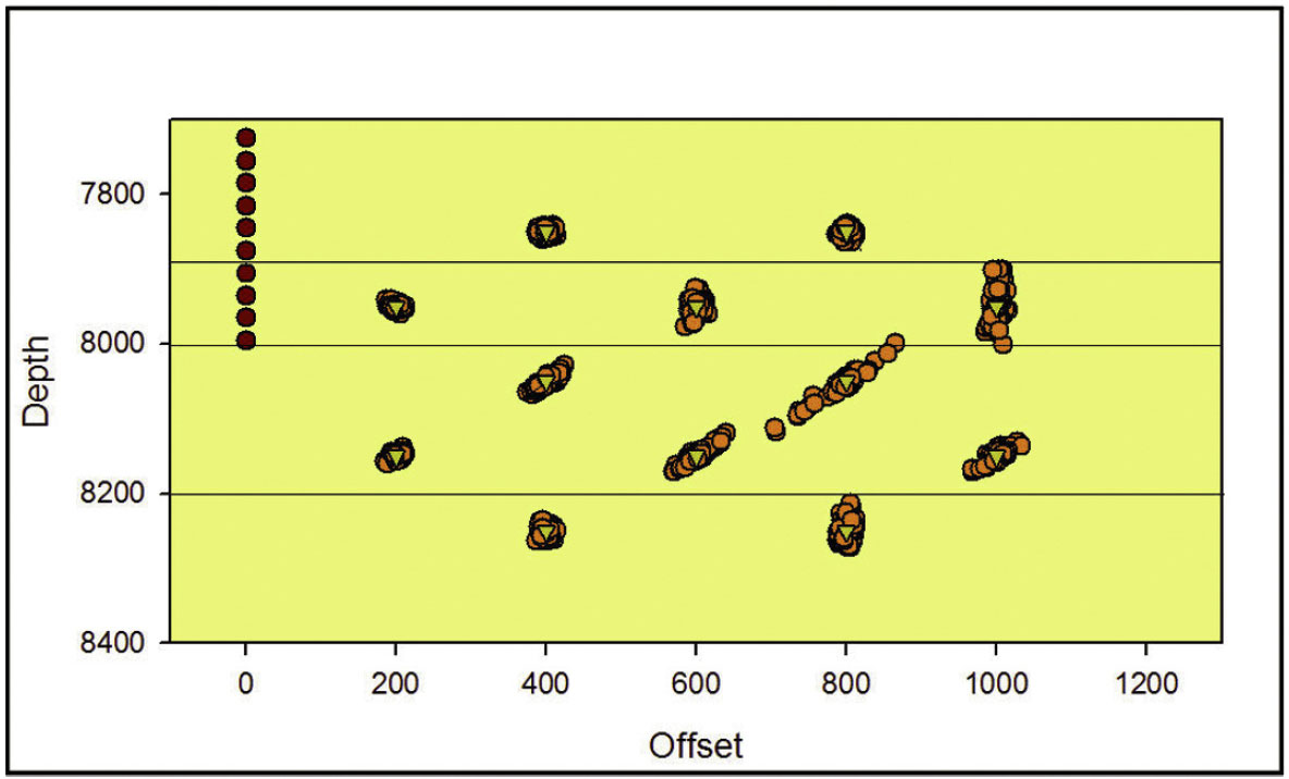
The event locations resulting from the Monte Carlo simulation sample the random location uncertainty resulting from the data uncertainties. Figure 3 shows the resulting locations which form ‘clouds’ that illustrate and define location uncertainty due to arrival time and directional uncertainty. The same velocity model was used for the forward model and the location calculations, so that the Monte Carlo event locations correspond to the random location errors without any velocity model errors. Notice that the individual ‘clouds’ can have different dimensions in different directions, which defines error ellipsoids representing the statistics of the location uncertainties (typically defined as one or two standard deviations of the uncertainty or Monte Carlo spread). In Figure 3, it is interesting to note the variability in location errors. For example, the depth uncertainty is greater for events in the shale, compared to above and below. Furthermore, the location errors generally increase with increased offset. Figure 3 shows another notable effect, whereby the cloud of events in the shale shows an inclined trend, related to the refracted travel paths.

To demonstrate the effect of an incorrect velocity model and the interaction with the random errors, the velocity in each layer was changed by 5% to produce a slightly more homogeneous model (Figure 1). This particular model was purposely assumed to accentuate the event location mislocation with this more homogenous model. The 5% variation is large compared to the normal uncertainty in the velocity model assuming good velocity model calibration, but was used here for simple illustration purposes to exaggerate the influence of the velocity model. Typically velocity errors could be associated with lateral inhomogeneities, changes in depth of the interfaces and anisotropy. Assuming the perturbed velocity model, the Monte Carlo simulation was repeated with the resulting locations plotted in Figure 4. The resulting events are systematically deeper, and in particular locations in the shale interval are particularly inaccurate with a cluster of events appearing closer to the sensor array. The event locations tend to cluster at the bottom of the shale, associated with the velocity interface.

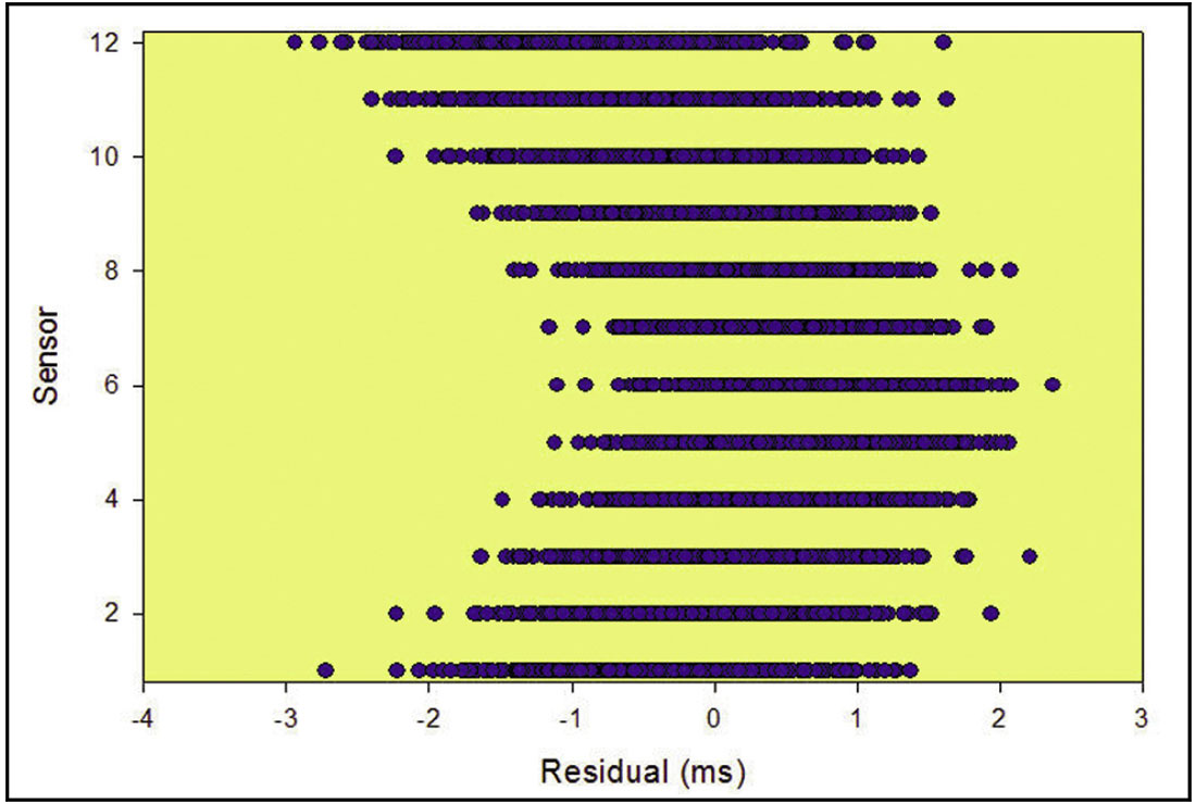
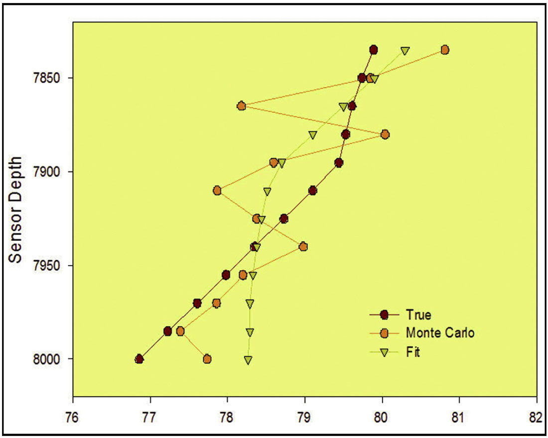
Based on the velocity model analysis, the potential for significant mislocations was identified if the velocity model was inaccurate. Since the creation of an accurate velocity model is often a processing challenge, this leads to a question of quality control of the velocity model. Beyond calibration with check shots and additional velocity measurements, the arrival time residuals (difference between ‘observed’ and theoretical arrival times from the computed location) through the sensor array also offer an important factor for quality control. Figure 5 shows the residuals for events located with the shale, which show a trend through the array consistent with an inaccurate velocity model, albeit here a significant velocity error was purposely assumed for demonstration purposes. At the upper and lower sensor (sensor number proportional to depth here) the computed locations result in negative residuals indicating that the velocity model is producing systematically late arrivals. This may seem non-intuitive since the assumed velocity model was created to be fast at the bottom of the array and slow at the top (Figure 1), but for the events in the shale the refraction through the velocity contrast at the top of the shale results in a specific moveout pattern that is attempted to be fit during the location procedure. This can be illustrated by considering in Figure 6, the p-wave arrival time moveout for one particular event in the Monte Carlo simulation. This particular plot shows an arbitrary example for the numerous iterations of the Monte Carlo, and is only included here for discussion purposes. Figure 6 shows the initially modelled arrival time curve (labelled ‘true’) which is then randomly perturbed during the Monte Carlo simulation and the theoretical moveout of the best fit location (labelled ‘fit’). Since the velocity contrast across the top of the shale at 8000’ has been changed the moveout at the bottom of the array is different which results in the systematic trend in the arrival time residual shown in Figure 5.

The moveout curve shown in Figure 6 is associated with the apparent velocity of the p-wave arrival of the waves through the array. Since the velocity model used for the source location is different from the model used to forward model, it is not surprising that the apparent velocity moveout curve does not match and has systematic relative errors/residuals. Linear borehole sensor arrays are a common microseismic monitoring geometry, and offer an ideal situation to calibrate the apparent velocity. The observed apparent velocity can be used to invert the velocity model, although the inversion is poorly determined a highly non-unique in many instances. Nevertheless, the arrival time residuals provide a means of quantifying the apparent velocity uncertainty which can be used for a sensitivity test or quantification of microseismic location uncertainty due to velocity model uncertainty.

Horn River Basin Model

A similar modeling exercise was performed for a velocity model approximating the Horn River Basin in NE BC (Figure 7). The Horn River is a relatively new shale gas play, with activity focused in both the Muskwa and Evie Shales. Similar to the Barnett, a relatively fast carbonate unit, known as the Keg River, underlies the shales. Another fast layer, the Mid-Devonian Carbonate lies between the two shale targets. Therefore, compared to the Barnett velocity model, the Horn River has additional complexity associated with two relatively slow layers with fast layers between and below. For purposes of illustration, two distinct geophone array depths were assumed. The shallow array, from 2255 to 2465 m is first assumed which would correspond to an array that could be deployed in an observation well completed in the Evie. In this case, a plug might be deployed in the MDC to provide pressure control in the Evie perforations and restrict the geophones to above the MDC. A second deeper array was assumed with sensors all the way down to the Keg River, which might be possible in a non-perforated well without pressure control issues.

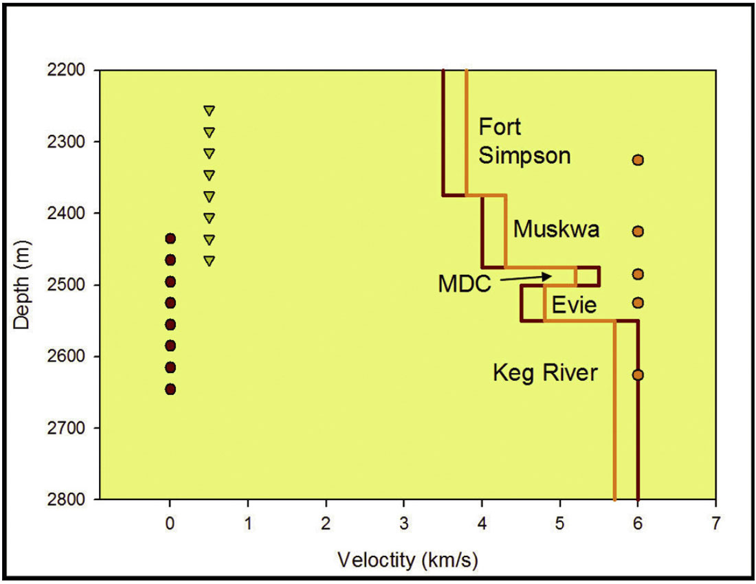
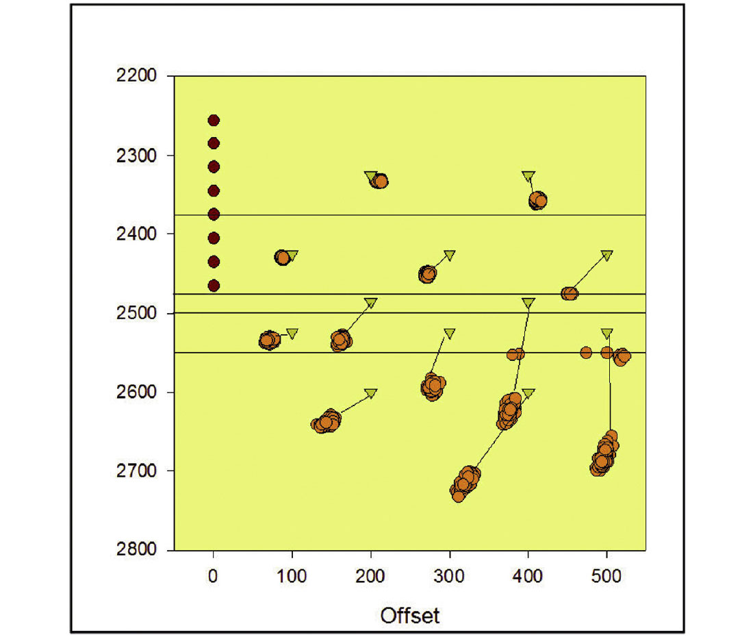
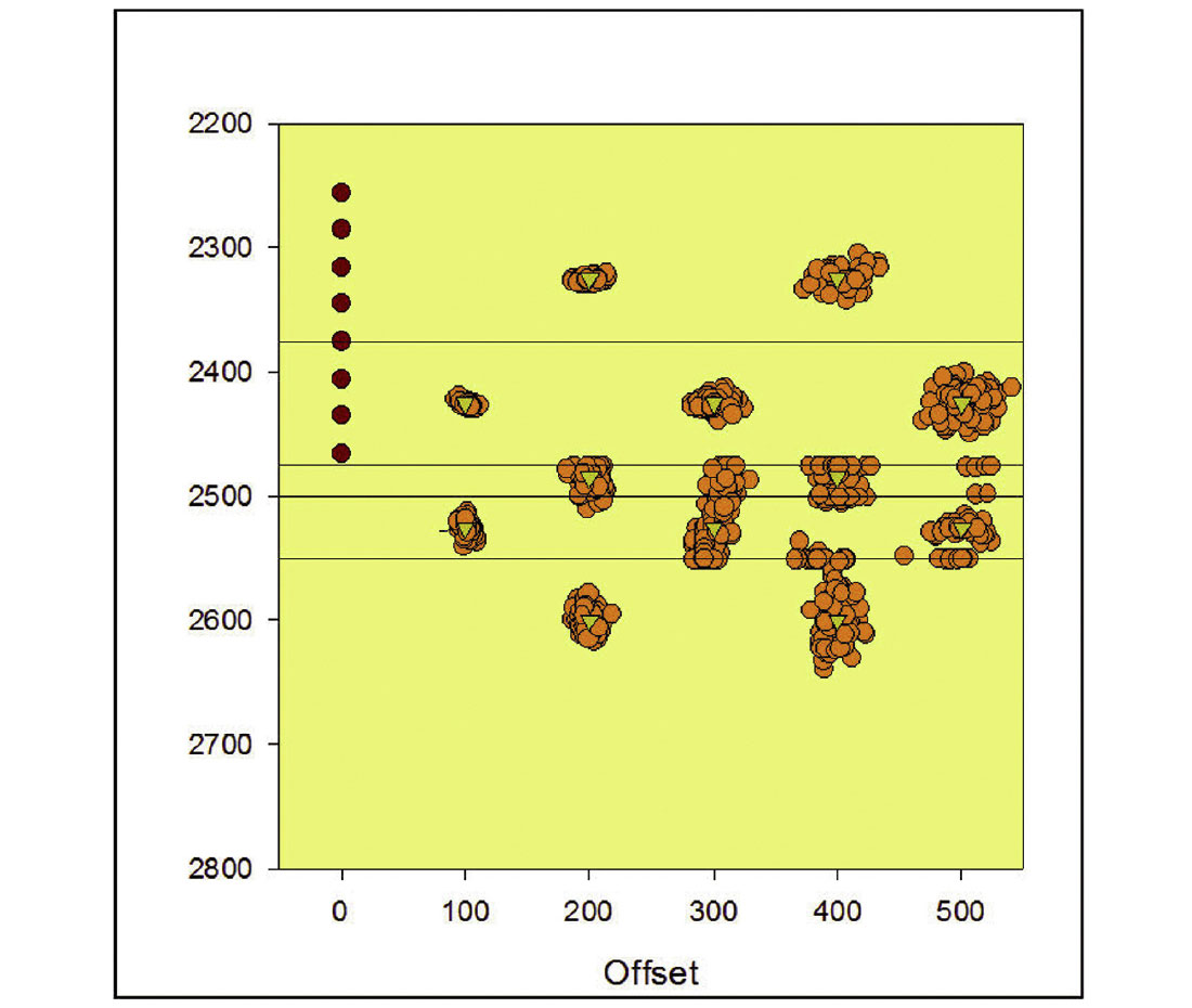
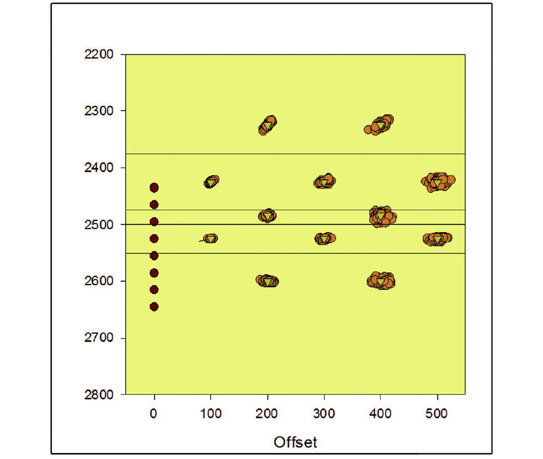
Figure 8 shows the Monte Carlo error estimates with the shallow array for a grid of points shown in Figure 7, offset out to 500 m from the monitoring well. Data uncertainty values and modeling and processing details were similar to those assumed in the previous example. Notice that the location uncertainties, especially in the vertical component, generally increase with depth. The greatest vertical error occurs for the deepest sources in the Keg River. By contrast the deeper array results in reduced vertical errors (Figure 9). The deepest sources in the Keg River still have the largest vertical uncertainty, but the uncertainties at all depths are significantly reduced. Clearly this represents a more optimal array position in terms of improved location accuracy. However, the complexity of the recorded seismic waveforms have not been considered here and would tend to be more complex, with possible critical refractions associated with the interfaces to the fast layers around the Evie. Waveform complexity could increase arrival time uncertainty resulting from coda from earlier phases and confident interpretation of various phases.

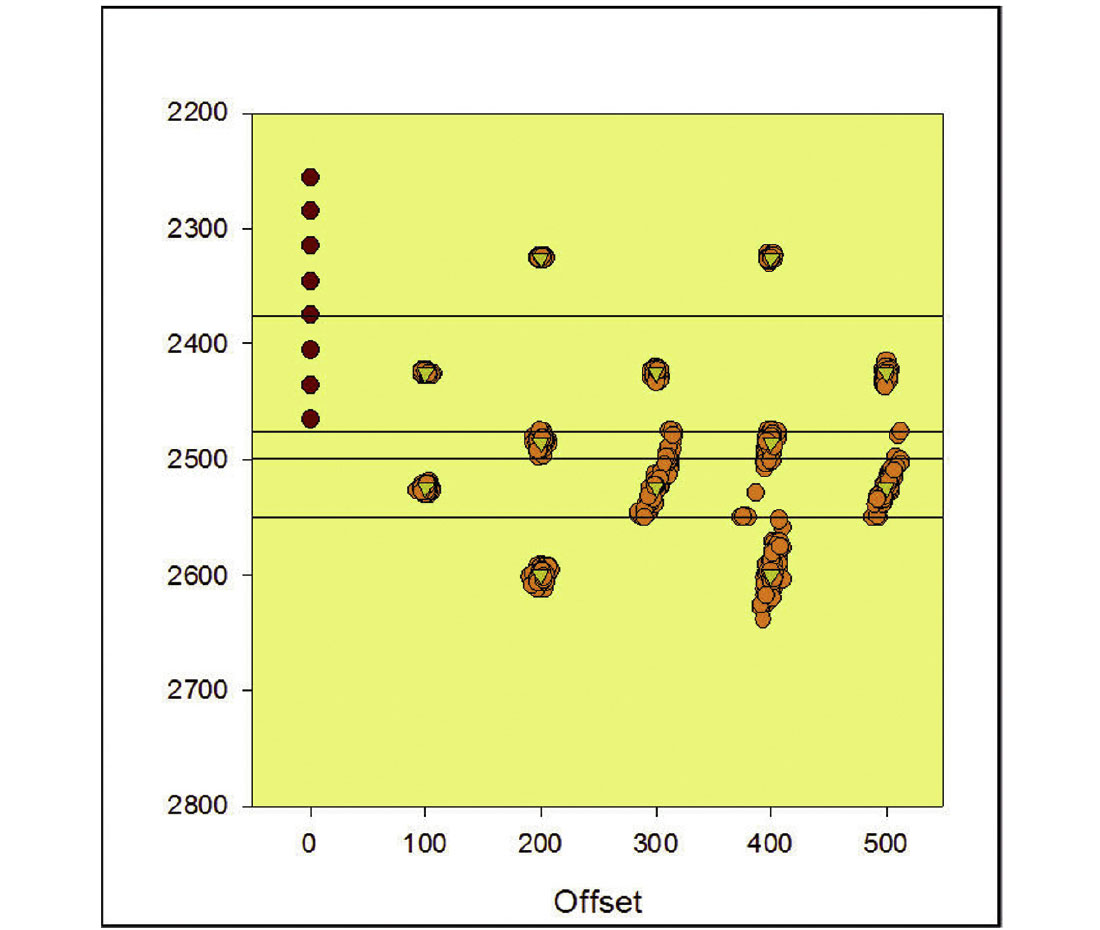
Next consider how the location errors respond to an incorrect velocity model (see Figure 10). As with the Barnett example, the velocity model errors could be assessed through apparent velocity errors in the arrival time residuals. Furthermore, a substantial relative velocity uncertainty of 5% has again been assumed for demonstration purposes, which exceeds probable velocity errors following confident velocity model calibration. Nevertheless, the Monte Carlo locations for the incorrect model with the shallow array is shown in Figure 10. The assumed velocity errors locate the events systematically too deep for all the source positions. However, other incorrect velocity models could be constructed that systematically mislocate the events to shallower depths. Most significantly, the source locations in the MDC are mislocated in the Evie for some of the Monte Carlo locations, although most are mislocated at a depth of approximately 2600-2700m in the Keg River. The sources in the Evie are mislocated near a similar depth interval in the Keg River. The sources in the Keg River are mislocated too deep. In summary, the shallow array can have substantial mislocations resulting from velocity model errors up to a maximum of about 150m.

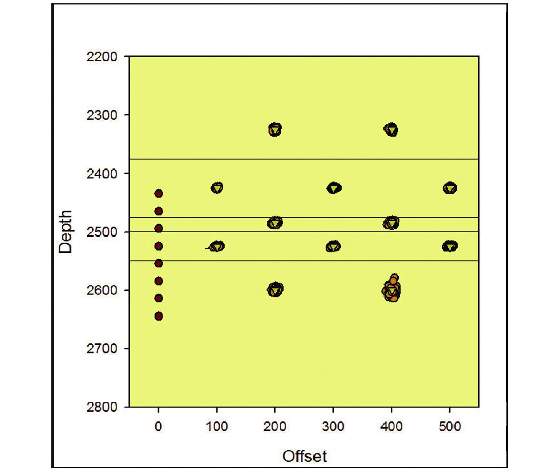
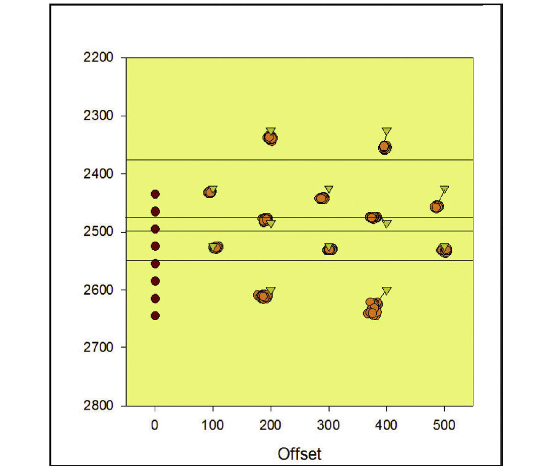
For comparison with the shallow array, consider the Monte Carlo locations for the deep array with the incorrect velocity model (Figure 11). The events are significantly more accurate with this array geometry, and also the spread of the Monte Carlo locations show significantly less random depth errors. The significance of this demonstration with the two array geometries, is that these two configurations show significantly different location uncertainties. The locations computed with the deep array are substantially more accurate, which leads to two implications. Firstly, this example points to the value of pre-monitoring modeling to assess location accuracy. Especially in cases where different array configurations or depth interval are possible, and the geometry is not overly constrained by practical completion constraints in a monitoring well. Secondly, these few examples lead to the possibility of optimizing the array position to maximize location confidence and minimize sensitivity to velocity model errors. Although this would require the definition of a target region, over which to minimize the locations. For example, hydraulic fracturing in the Muskwa may not lead to a concern with fracturing down into the Keg River and so optimizing location accuracy in the layers either side of the Muskwa may be of most interest.

Finally, to better quantify the potential location uncertainty for realistic velocity variations, a Monte Carlo simulation was performed with a 2% velocity variation simultaneously in each layer of the velocity model. No perturbations were made to the arrival time data in this specific simulation. A 2% velocity uncertainty is believed to better represent the accuracy of a reasonably well calibrated velocity model. Figure 12 and 13 show the resulting shallow and deep array locations, respectively. Note that these spread of locations represent the range of possible systematic event mislocations, and are more realistic and result in less uncertainty compared to the single 5% velocity shift described above. As shown previously the deeper array results in significantly less location uncertainty associated with the velocity model.

Conclusions

In this relatively simple modelling example, the influence of velocity model errors on location accuracy was demonstrated. The example shows that significant mislocation of microseismic events is possible if an incorrect velocity model is assumed. The example also demonstrates that arrival time residuals or systematic apparent velocity model errors are associated with an incorrect velocity model, which provides a convenient method of velocity model quality control by plotting arrival time residuals through the sensor array. An example based on the lithology of the Horn River Basin, demonstrates the variation in location uncertainty associated with different geophone array geometries.

Acknowledgements

Thanks to Mike Jones for useful comments.