Do you know what you think you know?

Long-time US Secretary of Defense Donald Rumsfeld once famously said that there are known knowns, and there are known unknowns. And of course there are unknown unknowns: “things we do not know we don’t know” (Rumsfeld, 2002). Perhaps there are unknown knowns too, though I’m not sure how you’d know.

When we think about uncertainty, we often think about the known unknowns—those are obvious. We worry about unknown unknowns, and we try to figure out what they might be. But we rarely think about the known knowns. They’re known, right?

Well locations are the cornerstone of a sound interpretation project. But anyone who has worked with subsurface data knows they can be problematic (Figure 1). Are you sure a given well location was loaded into the correct coordinate system? About 99% sure, you say, which is pretty darn good in this business. What about the directional survey? Was true or grid north identified correctly? Was the tool calibrated properly, with a recent declination? Was it properly interpolated, with the most appropriate algorithm for its geometry? Sadly, the only way to know any of this for sure is to dig up the well’s final report, and load all the data again.

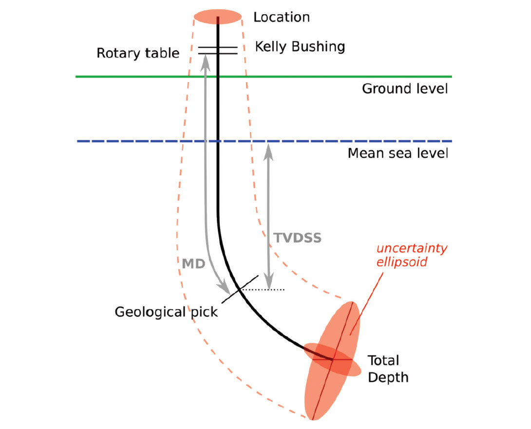
Perhaps the important thing is that it’s ‘accurate enough’. But how accurate is it, and what is ‘enough’? Is the bottom hole location correct to within 1 m? 10 m? 100 m? If you’re like me, you have no idea, and the cost of finding out is too high.

Well location has implications for an interpretation workflow that is sometimes rushed and, in my experience, usually not done very scientifically: well-to-seismic calibration. This workflow, the one I most often hear Chief Geophysicists worrying about, is fraught with opportunity for error. The replacement interval is often mishandled. Log editing is a minefield, and stretch-and-squeeze is similarly explosive missile testing range. I have rarely seen a checkshot survey loaded correctly: usually the datum is not the same as the seismic datum, and the correction has been botched, if it was applied at all.

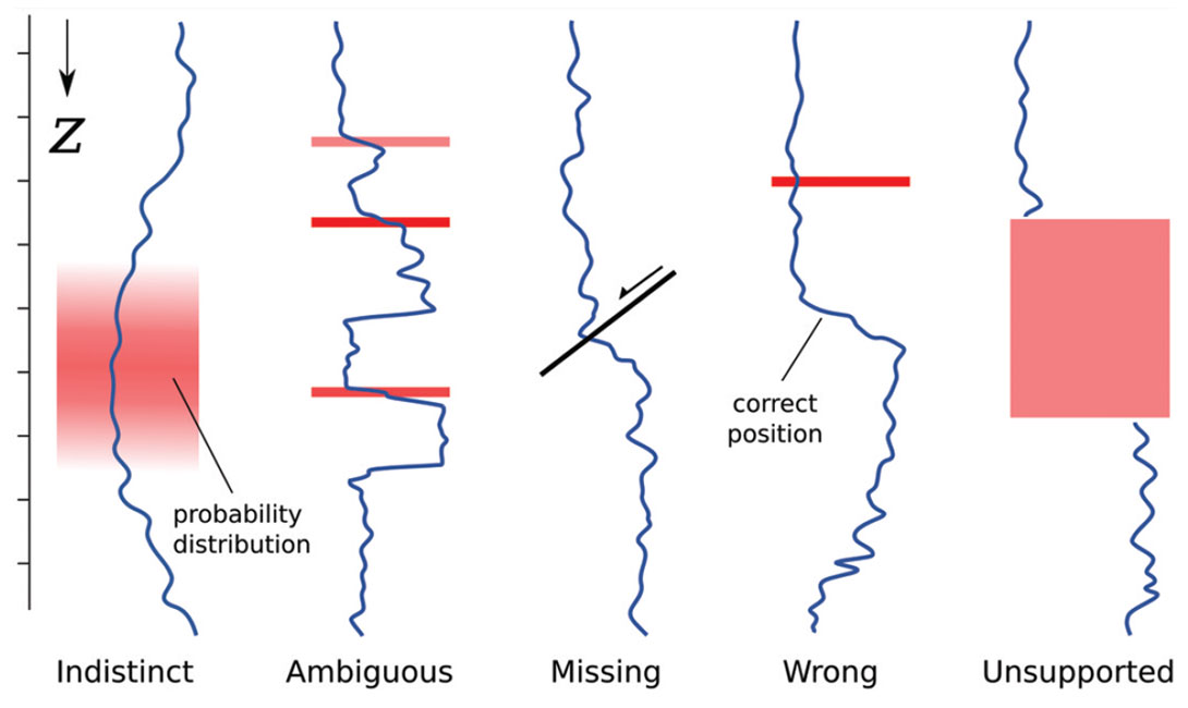
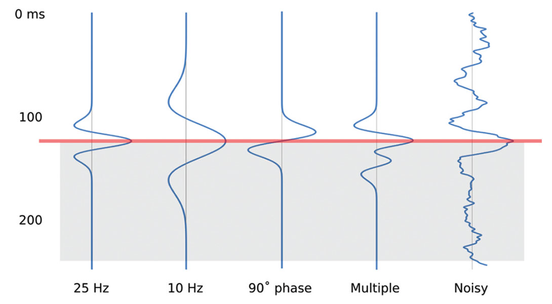
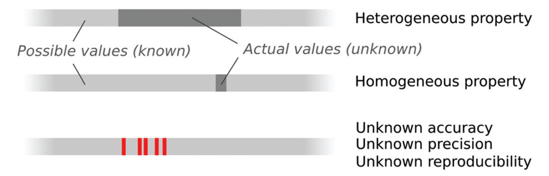
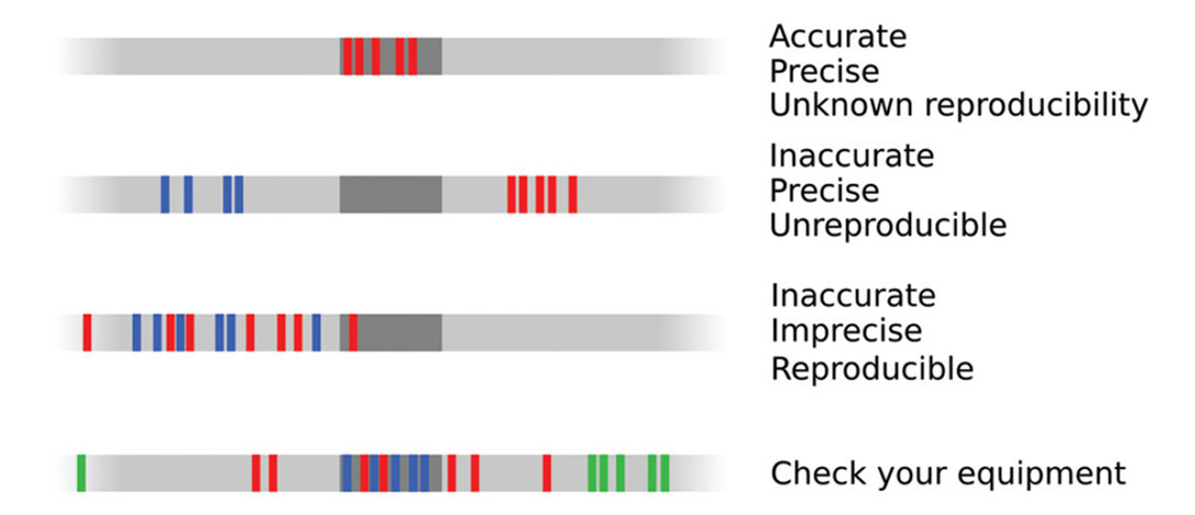
The rest of the data in our well tie are corrupted too. The well logs contain errors, inaccuracy, and bias. The picks we make are at risk in all sorts of ways (Figure 2). The seismic data we wish to calibrate, and the interpretations we make in them, are equally soaked in fuzziness (e.g. Bianco, 2011)—see Figure 3. Clearly, we have a problem.

Problems of uncertainty

Charles Dudley Warner said, “Everyone complains about the weather, but nobody does anything about it.” I think you could say the same about subsurface uncertainty. Sure, we build it into our geomodels, but what about dealing with it before the geomodel? Or, more importantly, after? Do we actually make decisions within a robust probabilistic framework?

I think there are some strange things about our particular problems that make them difficult to work with. For one thing, probabilities are difficult, unintuitive concepts for most people (e.g. Hall, 2010). It’s almost impossible to think about them without deep thought, discussion, and a computer.

Another problem is that it’s not always clear what we’re forecasting. Unlike predicting the weather or a roulette wheel, we are in the business of ‘predicting’ things which have already happened, usually a very long time ago. When we drill a well, it’s more like opening Schrödinger’s box than rolling a die: the probability density function collapses when the bit penetrates the reservoir.

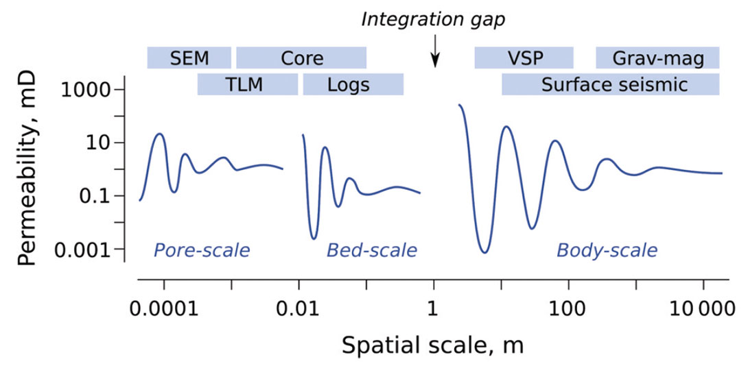
Scale is a confounding factor. Quantitative uncertainties are inextricably bound up with the scales of our measurements and of our models. For example, Figure 4 illustrates the socalled Representative Elementary Volume for various model scales (Bear, 1972; Ringrose et al., 2008). The concept sounds complicated, but is intuitive for geoscientists: all rocks are microscopically heterogeneous, but above some characteristic scale we can assume that pore-scale properties approach a constant value. At larger scales, bed-scale properties fluctuate, then stabilize, and so on. The idea is that at some sufficiently large scale, we can treat any rock as a homogenous medium and model it with a single cell. The catch is that we have to collect enough data to validate this scale change. What is ‘enough’? You need to be able to model spatial variance at the target scale of the geomodel.

Finally, scale manifests itself in another way: the integration gap (Hall, 2011). Figure 4 shows that there is a lack of scale overlap between sample- and well-based measurements at the small scales, and seismic imaging methods at the large scales. This is one reason why seismic-to-well calibration is so pivotal a workflow, and why integrated interpretation is so key, and so hard. The gap spawns substantial uncertainty as we struggle to reconcile the various datasets with the REVs.

The one thing we know for sure about our interpretations and predictions of the subsurface is this: they are wrong. What’s more, you’ll ever know the true answer, because all we can ever do is interpret a tiny amount of filtered data. It would seem to be a miracle that we get anything done at all. Of course we do, but we’d like to get better at it. The fact is, most wells are poor performers.

Types of uncertainty

Broadly speaking, we can describe two classes of uncertainty (National Research Council, 2000):

Class A
Statistical uncertainty, sometimes called aleatoric, structural, external, objective, inherent, random, or stochastic uncertainty. Errors in this category change each time we measure something. They should be the same for equally competent experimenters. They are unavoidable, at least beyond some limit of irreproducibility, but can be modeled with statistics.

Class A
Conceptual uncertainty, sometimes called epistemic, functional, internal, subjective, or knowledge uncertainty. Such an uncertainty is knowable in principle, but not known in practice. Gaps in knowledge, model inadequacy, differences of expert opinion fall into this category.

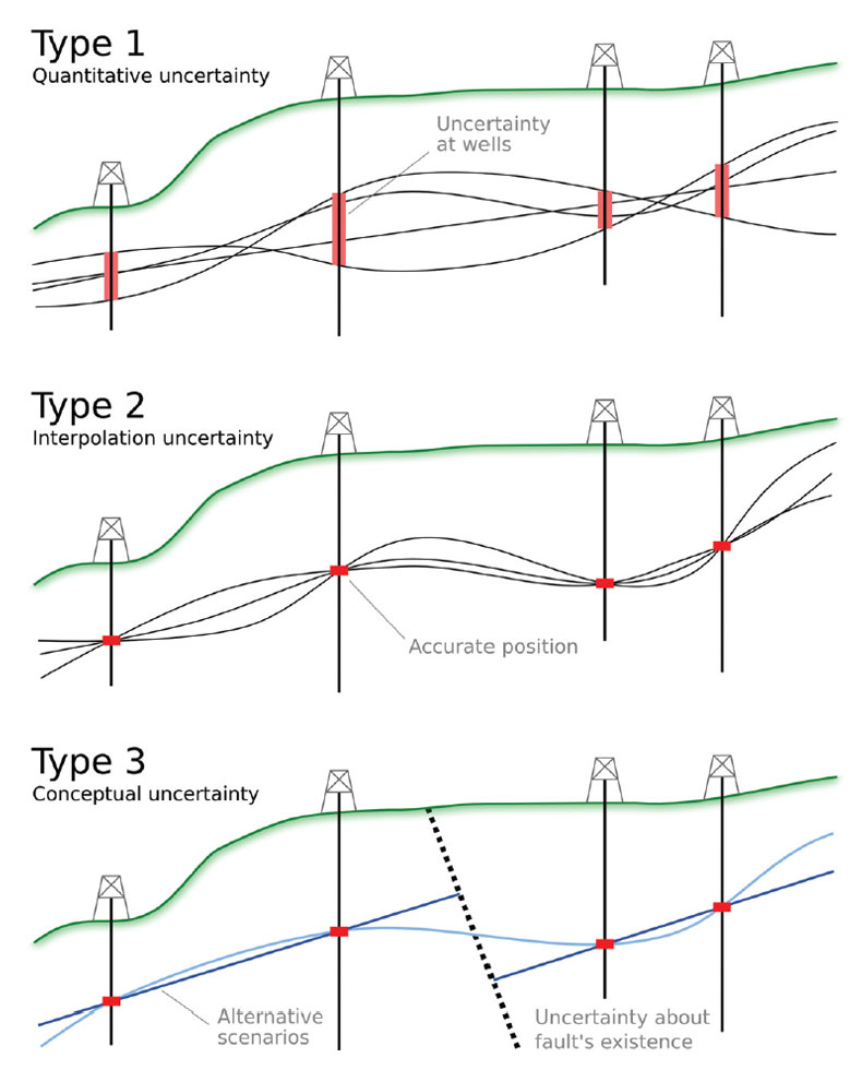
I find these classes rather difficult to grasp. They seem vague and too general. Mann (1993) was more practical. He wrote on geological uncertainty and used the following scheme, adapted somewhat by Wellmann et al. (2010) and illustrated in Figure 5:

Type 1
Quantitative uncertainty in known information. For example, error in data points, compounding imprecision, inaccuracy, and irreproducibility (Figures 6 and 7). In general, I think we all know these errors and uncertainties infest our data, but it’s rare to see anyone capture them in a rigorous way. Usually, they are characterized by some fudge factor: perhaps I allow well picks to vary by ±5 m in a geocellular model, for example. Sometimes these errors are synthesized in crossplots and histograms, resulting in a more robust estimate of error. In principle, at least, these errors are knowable, though they may be irreducible. Better instruments and methods should reduce them maximally. These belong in Class A.

Type 2
Quantitative uncertainty in models of unknowable information. A type of Class B uncertainty. A model might be a grid, an approximation, or a gridded surface. For example, if we think about structural modeling, this might mean interpolation and extrapolation of stratigraphic surfaces. If you use deterministic mapping methods, then this uncertainty is not represented at all: the structural framework for the geomodel is usually determined to be the ‘most likely’ or ‘best technical’ case. Most geomodellers do try to capture Type 2 uncertainty for reservoir properties, however, realizing manifold distributions. Then again, how many of those models are flow simulated is a practical issue, not a statistical one, because flow simulation is much slower than property simulation. For similar reasons, the parameters of the stochastic models are usually not themselves subject to perturbation.

Type 3
Qualitative uncertainty about the state of nature. Again, this is Class B. I tend to think of this as uncertainty about the conceptual geological model in exploration, or the velocity model in seismic processing, or the geopolitical climate in project planning. The uncertainty can be profound, as demonstrated by the eye-opening study by Bond et al. (2007). Any time you need to think about scenarios, or ask yourself which path you need to take, you are probably dealing with Type 3 uncertainty. As an industry, I think we usually ignore this, feeling like it is better to use our professional judgment and pick the most likely scenario. Indeed, we are often pushed to do this by management: “if you had to pick one, which depositional model would you go with?”. I think this is because the only way we know to handle Type 3 uncertainty is to build another scenario, essentially doubling the work of picking one and running with it.

Things we can do

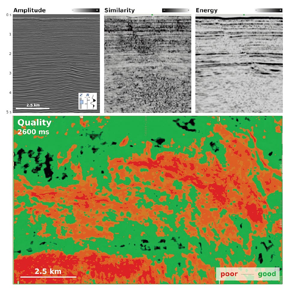
Quantify all the Type 1 errors that you can. Quantify them. Even if you don’t use them, at least you’ll know what they are: critical information when risking prospects. Try using them to constrain models and reality-check distributions. Try to estimate the reliability of things you normally take at face value. I like to try to judge the reliability of seismic data with a combinations of attributes (Figure 8), which you can corroborate (or not!) with your subjective opinion.

Ask laboratories for Type 1 error data. Provide enough samples to represent the natural variability at scales you are interested in. Ask them to test against known standards and do repeatability tests, perhaps by secretly providing the same samples multiple times. Remove the possibility of unintentional bias by blind labelling.

Deal rigorously with Type 2 errors. This means playing with the parameters in your gridding and property modelling tools. The tools and workflows exist, it just takes time. Explore what happens if you perturb the cementation exponent in Archie’s equation. Talk parameter selection over with your colleagues, being clear about the implications of the choices you make. These uncertainties drive the shape of your final distribution.

Catalog Type 3 errors, even if you don’t deal with them. By all means choose a scenario, but don’t deny the possibility of being wrong. At least think about the most important ways in which you might be wrong. Ask others. Look at previous interpreters’ work. Argue your case—it helps explore the evidence—but don’t treat conflicting models as challenges to beat down. They may be valid points in the solution space.

Embrace iteration as an opportunity. I believe the tendency to think in terms of time-limited projects, and to talk about ‘final interpretations’ and so on, draws us into the idea that our answer is final. In fact, unless you happen to be working on a fleeting opportunity, our interpretations are almost always temporary, being revisited at some point in the future, perhaps quite soon. Recognize that all you are trying to do is be more nearly right than yesterday; you aren’t trying to be (and can not be) completely right.

The next paradigm

Full disclosure: I am way out of my depth here. It may be best to think of this section as geoscience fiction. But science fiction can help us imagine a better future, so maybe we can think about how we will move beyond today’s pseudo-stochastic paradigm.

I think representing Type 1 and Type 2 uncertainty should be easy. But doing a rigorous job will require a new type of data model. As well as putting tables of data in the database, we need to add tables of uncertainty. Think of it as adding a new axis, or dimension, to the database: every single table needs a set of sister tables, showing some representation of the precision, accuracy, and reproducibility of every data item. In many cases, it may be possible to model the uncertainty: precision can be statistically modelled, accuracy can be measured by frequent calibration against standards, reproducibility can be checked. In other cases, we will have to make assumptions. We’re not storing data as such, we’re storing haze. Haze is a multi-scale meta-attribute with a finite, non-zero value for every element in today’s database.

Type 3 uncertainty is a harder problem. There seems to be no way around having to do a lot of work twice in order to capture different models. The one opportunity I am sure we are missing is the exploitation of legacy interpretations. If the database and hazebase contain yet another dimension—time—then perhaps we can use clever versioning to keep track of internally-consistent interpretation assets, as well as how they develop over time. Later interpretations, for example, will likely be supported by more or better data, and could therefore be considered more reliable. Perhaps the interpreter’s experience and the time spent on the analysis are factors. The present synthesis can combine the various scenarios, with their various reliabilities and a priori likelihoods, into straightforward probabilities using well-known Bayesian methods.

The problems really start when we want to do calculations with our multi-dimensional data-, haze-, and time-base. Computers are fundamentally deterministic. If we want stochasticity, we have to fake it with tools like Monte Carlo simulation. So if we want to model 1000 rolls of a die, for example, we make 1000 rolls of an imaginary die, faithfully recording each outcome and thus building a histogram of results. (We wouldn’t really do this for such a simple problem, but as we combine parameters, Monte Carlo simulation becomes the only reasonable path). Doing these calculations with haze would take an unpractical amount of time.

Instead, we need quantum computing. This nascent technology will let us compute not with binary (on-off) bits, but with uncertain, multi-valued qubits. Uncertainty is built-in to the method, and comes for free. Quantum computers will not need Monte Carlo methods to simulate uncertainty, but will simply model it directly. There are quantum computing simulators out there (look for quantiki.org), as programmers prepare to control these future machines. With luck, quantum computing chips will be solving hard problems like ours within the decade.

Conclusions

Uncertainty affects everything we measure, interpret, and model.

There are three basic types, and it helps to recognize them and treat them accordingly. They are: stochastic uncertainty in our data, uncertainty about interpolation, and uncertainty about the overall state of nature.

We can improve our handling of uncertainty with some simple steps:

• Quantify all the Type 1 errors that you can.
• Ask laboratories for Type 1 error data.
• Deal rigorously with Type 2 errors.
• Catalog Type 3 errors, even if you don’t deal with them.
• Embrace iteration as an opportunity.

I’m looking to quantum computing for profoundly improved uncertainty handling.

Acknowledgements

Thank you to Evan Bianco for conversations leading to this article, and for reviewing the manuscript. This work is licensed under the terms of Creative Commons Attribution. You can find all the figures at www.subsurfwiki.org.