The magic of Lamé

IF GEOPHYSICS REQUIRES MATHEMATICS FOR ITS TREATMENT, IT IS THE EARTH THAT IS RESPONSIBLE NOT THE GEOPHYSICIST.
-Sir Harold Jeffreys

This quote was offered as a disclaimer on a course I took at the University of Calgary in 1988: Dr. Ed Krebes’ Geophysics 551 Seismic Techniques. This excellent course was pivotal in my enlightenment regarding Lamé’s parameters. I repeat the quote here as it disclaims my seemingly unnecessary obfuscation in the use of equations that follow.

The basic earth parameters in reflection seismology are P-wave velocity VP, and S-wave velocity VS. However, these extrinsic dynamic quantities are composed of the more intrinsic rock parameters of density and two moduli terms, lambda (λ) and mu (μ), introduced by the 18th-century French engineer, mathematician, and elastician Gabriel Lamé. Lamé also formulated the modern version of Hooke’s law relating stress to strain as shown here in its most general tensor form:

Here, σ_ij is the i-th component of stress on the j-th face of an infinitesimally small elastic cube, c_ijkl is the fourth rank stiffness tensor describing the elasticity of material, ε_kl is the strain, and δ_ij is the Kronecker delta. The adage ‘stress is proportional to strain’ was first stated by Hooke in a Latin anagram ceiiinosssttuv, whose solution he published in 1678 as Ut tensio, sic vis meaning ‘As the extension [strain], so the force [stress].’ Despite being interestingly reversed and non-physical, Hooke’s pronouncement is illustrated here with complete mathematical rigor, and this equation creates the basis for the science of materials, including rocks. Interestingly, and most notably, only Lamé’s moduli λ and μ, appear in this equation; not bulk modulus, Young’s modulus, Poisson’s ratio, V_P, V_S, or any other seismically derived attribute.

The methods to extract measurements of rocks and fluids from seismic amplitudes are based on the physics used to derive propagation velocity. This derivation starts with Hooke’s law and Newton’s second law of motion, and yields a set of partial differential equations that describe the progression of a seismic wave through a medium. It also forms the basis of AVO-based descriptions of the propagating medium.

The P-wave propagation of a volume dilatation term θ derived from Hooke’s law is:

and the S-wave propagation of the shear displacement term (d # ush):

The vector calculus in these equations says that the particle or volume displacement for a travelling P-wave in the earth is parallel to the propagation direction (as d # i = 0), whereas the particle displacement imposed by a passing S-wave is orthogonal to the travelling wavefront. Consequently, the intuitively simple Lamé moduli of rigidity μ and incompressibility λ afford the most fundamental and orthogonal parameterization in our use of elastic seismic waves, thereby enabling the best basis from which to extract information about rocks within the earth.

These Lamé moduli form the foundation for linking many fields of seismological investigation at different scales. Unfortunately the historical development of these fields has led to the use of a wide and confusing array of parameters, which are usually complicated functions of the Lamé moduli. None of these are inherent consequences of the wave equation, as the Lamé moduli are. This includes standard AVO attributes such as intercept and gradient or P-wave and S-wave reflectivity that are ambiguous and complex permutations of Lamé moduli λ and μ, or Lamé impedances λρ and μρ. Many other parameters such as Poisson’s ratio and Young’s modulus have arisen due to inappropriate attempts to merge the static un-bound domain of geomechanics to the dynamic bound medium of wave propagation in the earth. These attempts have resulted in the use of contradictory assumptions, which are completely removed when restating equations using the magic of Lamé moduli.

Q&A

You pioneered the development of the LMR attributes in 1997. After 17+ years of its applications in the seismic world, what do you have to say?

My motivation for introducing LMR back in the 90’s has endured I believe due to the insight and improved understanding of extrinsic velocity or impedance measurements afforded by recasting these quantities in the more intuitive intrinsic rock parameters of density (ρ) and the orthogonal Lamé moduli terms of shear rigidity mu (μ) and incompressibility lambda (λ).

Recasting the basic dynamic earth parameters of P-wave velocity and S-wave velocity in Lamé parameters both simplifies and offers new insight into the rock property factor M/ρ (where interestingly M is either μ or λ + 2μ and not any other modulus in common use such as Young’s or Bulk modulus or even Poisson’s ratio) that controls and is a consequence of seismic elastic wave propagation.

Despite what I thought was an obvious advantage to using the LMR approach, standard AVO methods continue to be applied to extract attributes such as intercept and gradient, P-wave and S-wave reflectivity or Vp/Vs velocity and Poisson’s ratio. These attributes are far more ambiguous as they contain complicated permutations of λ and μ or Lamé impedances LambdaRho λρ and MuRho μρ.

(Relations for λ = (Vp² – 2Vs²)ρ² and μ = Vs²ρ² while λρ = Ip² – 2Is² and μρ = Is² where Ip and Is are P-wave and shear wave impedances)

Even at the static engineering lab scale a given material has various moduli that are purely a function of measurement conditions combining a complex mix of invariant λ and μ that form the basic elements within these moduli e.g.

and

The bulk modulus kappa (κ) in particular, requires some clarification as it is used in Biot-Gassmann fluid substitution by being embedded in the P-wave velocity and is considered to represent incompressibility, while λ is undefined, being generally termed as just the first Lamé parameter. In 1999 and 2002 I gave two courses on AVO where I showed that the fluid term Δλ that controls the FRM (fluid replacement modelling) in Biot-Gassmann equation can be very closely approximated by

where Δλ is the difference between the saturated and dry pore space modulus of Hedlin et al. (2003), λfluid is the fluid modulus, Δκ is the difference between the solid and dry bulk modulus and κ_solid the solid bulk modulus. Some useful observations that can be seen from this simplification of the Biot-Gassmann equation are:

• Low Δλ sensitivity for high modulus (κ_solid) rock e.g. carbonates
• λ can never be negative as λfluid, φ, Δκ² and κ_solid² are always positive
• Can we find a specific Δλ AVO fluid signature?

Finally in the face of considerable resistance and controversy, I consider λ to be a pure, unambiguous and true measure of incompressibility, as it relates normal axial and lateral strain to uniaxial normal stress (as shown by the strain dilatation term θ in Hooke’s law). Consequently λ is primarily a longitudinal or normal quantity and therefore orthogonal (i.e. independent) to μ a quantity that relates a transverse shear stress to shear strain. This is not the case for the volumetric bulk modulus κ since it implicitly relates to a measure of shear strain, hence the shear modulus μ, due to the volume’s change in shape resulting from triaxial or hydrostatic stress.

Furthermore Lamé parameter λ is considered to be pure incompressibility and not the bulk modulus κ, as λ is the only modulus involved in both the hydrostatic stress-strain relationship and acoustic wave propagation for a fluid (i.e. where rigidity μ vanishes). In addition to these Lamé parameters λ and μ two new attributes LambdaRho λρ and MuRho μρ (Lamé impedances) are obtained from AVO by using moduli and density relationships to impedance. An improved identification of reservoir zones is possible by the enhanced sensitivity to pore fluids from pure incompressibility λ or λρ. Furthermore a better understanding of lithologic variations independent of fluid effects, such as sand/shale ratio can be obtained by analysing fundamental changes in rigidity μ, incompressibility λ, and density ρ parameters as opposed to a mixture of parameters within seismic velocities or impedances.

Some geophysicists opine that as the derivation of these attributes involves squaring the P- and S-impedance attributes, any error in these gets magnified in the estimates of LMR attributes. How do you react to that?

Yes, there has been considerable debate about this, but again most of the arguments are not valid being based on very cursory assessment of the effects of squaring and subtracting P-wave and S-wave impedances (Ip and Is respectively). First of all the squaring causes an expansion (almost a doubling) of the cross plot space going from impedance (Ip vs. Is) to LMR (λρ, μρ) with obvious advantages for a number of reasons such as:

a) improved identification of reservoir zones by the enhanced separation and sensitivity to pore fluids from λρ

b) there is a specific correlated direction and range for the error that is not random because the inversion for P-wave and shear impedance are correlated (high with high, low with low; see Cambois (2000, 2001) and so the error analysis appears as (Goodway, 2001)

Using the Vp and Vs shale values as in Table 1 above taken from log data in the Glauconitic channel play of Southern Alberta, along with Vp and ρ errors of 1% gives a dλ/λ error of 1.1 % from equation above and this is now similar to the original Vp and ρ errors and much less than both Vs and μ errors.

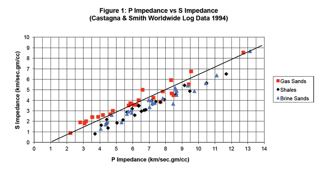
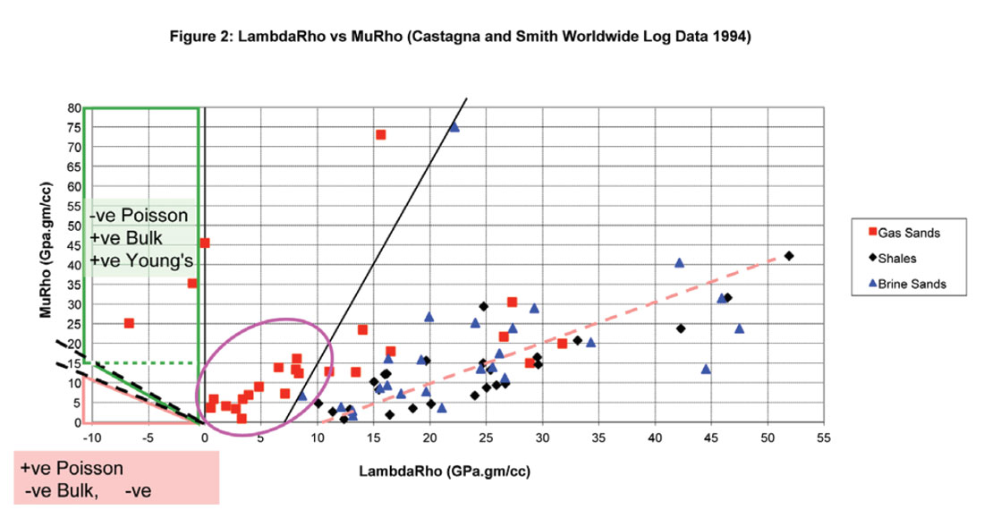
Continuing with this analysis of various moduli and AVO attribute sensitivity and error detection, the following graphed Figures 1 and 2, compare Castagna and Smith’s (1994) published world-wide logs plotted as P-impedance versus S-impedance compared to the equivalent LambdaRho versus MuRho cross-plot. A number of interesting observations can be made by comparing the cross-plots:

1. There is clearly a better separation of the gas sands from brine sands and shales in the λρ, μρ cross-plot as all the space is now available for lithology and fluid characterisation. This is not the case for the equivalent impedance cross-plot that shows a strong narrow correlation between Ip and Is for all rock types giving rise to relationships such as Castagna’s “Mudrock Line” (dark lines show cut-offs for gas sand separation on both cross-plots). The reason for this strong Ip to Is correlation stems from the same ambiguity in the Vp, Vs velocity relationships that share rigidity Mu as mentioned above. By contrast the λρ, μρ values are fundamentally more orthogonal giving rise to both tight clusters of similar lithologies (lower left quadrant gas sands as circled) as well as distinctly separated linear relationships for background brine sands and shales (dashed orange line).
2. There is a more intuitive interpretation of these rock types in λρ, μρ cross-plot space, where the circled low μρ gas sands are most likely younger, less consolidated sands than the three gas sand values that appear well separated in the upper left quadrant (high μρ range).

However, a major error is missed here, both by Castagna and in the contested response and exchange with George Smith (of Smith and Gidlow repute) as published in Geophysics letters to the editor. The error concerns 3 of the gas sand values # 3,4 and 6 that Castagna published as they have zero or negative Lambda (but positive bulk modulus) values indicating that the logs are in error. Furthermore as these three isolated points have positive bulk and Young’s moduli so the values could be used for modelling by Gassmann fluid substitution without any thought to the possibility that the logs are in error. Even further confusion would arise if any of the low μρ gas sands were to fall in the negative Lambda region shown by the lower left orange triangle, then Poisson’s ratio would be positive and believable while the bulk modulus, Young’s modulus and Lambda would be negative. My conclusion from the λρ, μρ cross-plot mapping of the confusing positive to negative non-linear behaviour for bulk, Young’s moduli and Poisson’s ratio within the clearly consistent negative Lambda region, is that Lambda alone represents the material’s true incompressibility and the other parameters disguise measurement errors.

I was the only person who noticed this error back in 1997 and remain so to this day as a Vp/Vs analysis alone continues to mask these log points, evidenced more recently by other authors who have used the dataset even with titles such as “AVO ritualization and functionalism (then and now)” (Ross, 2010). The only way I noticed was by transforming Vp vs Vs or Ip vs Is to LambdaRho vs MuRho as shown in Figures 1 and 2.

For the unconventional resource characterization, you have gone ahead and implemented the horizontal confining stress in terms of closure stress scalar, which is given in terms of the λ and μ parameters, and some others. What is your take on the determination of sweet spots with regard to the brittleness and TOC, in terms of the λρ and μρ templates you work with or with Young’s modulus and Poisson’s ratio? How do they compare? Do you think this is working adequately, as is being practiced in the industry, or something more has to be done?

Well, first let me briefly review the theory of the minimum closure stress equation expressed in seismic or LMR form for some insight into the physical meaning of the terms. Figure 3 below, from a slide I have shown at various technical meetings, captures the transformation of the engineering closure stress equation (upper equation in terms of ν and E) to its LMR form (lower equation in terms of λ and μ). The first thing to notice is that there are two confining (perpendicular) stresses the vertical effective overburden stress (maroon box) and the horizontal stress due to the tectonic term (purple box). These are both rotated into the direction of the effective minimum horizontal stress (or closure stress) by the closure stress scalar (CSS) or what I prefer to call the Bound Poisson’s ratio. My reason for this nomenclature is that the model for the fracture plane being considered (as shown schematically to the right) is that of “Plane Strain” i.e. there are no horizontal strains (e_x, e_y) in x and y just stresses σ_x σ_y. This means that the rock is bound hence the term Bound Poisson’s ratio for λ/(λ+2μ) which is actually just one λ short in the denominator from the more familiar Unbound Poisson’s ratio.

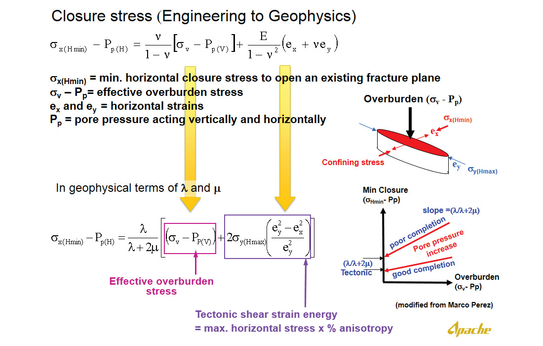
The insight gained from the LMR reformulated equation is that the horizontal tectonic term acting in the y-direction is in fact a function of a shear stress whose perpendicular effect is to confine (increase) the minimum horizontal closure stress (x-direction) as a function of the elliptical strain energy eccentricity (ey² – ex²)/ey² of the idealized fracture shown in the model cartoon to the right of Figure 3. The impact of these various stresses, differential horizontal strain energy, pore pressure and the CSS can be understood by cross plotting the effective minimum closure stress against the effective overburden stress as shown in the graph at the bottom right of Figure 3. From this the minimum closure stress equation can be seen as a linear relation with the intercept representing the horizontal tectonic term (scaled by CSS) and a slope equal to the CSS. So a lower intercept and slope is better while moving to the origin on the lines of constant CSS indicates an increase in pore pressure.

Moving on to the following questions, Figure 4 shows a petrophysical log based LMR template that demonstrates the correlation between CSS, ν and E to engineering parameters such as the instantaneous shut in or break down pressure per frac stage and estimated ultimate production (EUR) that we use to seismically map “sweet spots” and hence optimize completions or better still to place pads. The circular and square data points are inverted LMR values extracted at specific stages color coded by EUR/stage and break down pressure within the Muskwa/Otter Park zones in the Horn River Basin. The template is somewhat busy but captures a lot of information, demonstrating the differences between λρ and μρ to ν and E for an improved discrimination and understanding of brittleness and the effects of pore pressure and TOC not considered by geomechanics.

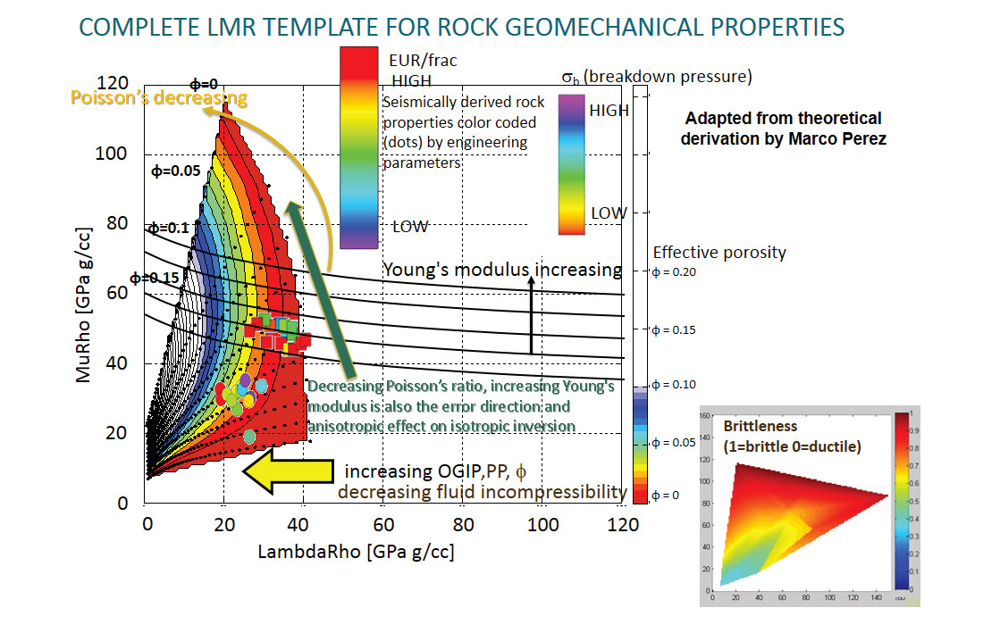
The following general observations can be made. Gas shales occupy a space away from ductile shales due to their higher quartz content giving an increase in shear rigidity μ (or μρ) and a decrease in Poisson’s ratio hence CSS. However, μρ and Poisson’s ratio alone do not clearly distinguish gas shales from ductile or calcareous shales that are barriers to frac stimulation, as they share a similar narrow range of values e.g. the square data points in the template. A more significant observation is that a decrease in incompressibility λ or better still λρ is the best discriminator of gas shales from ductile shales, unfracable calcareous shales and carbonate lithologies. This is clearly seen by the horizontal shift parallel to the LambdaRho axis (yellow arrow) with a near doubling in relative EUR values shown by the colored circular data points. Beyond this and less well known is that a decrease in λρ shown by the yellow arrow is an indicator of the following key attributes for the best gas shale zones:

1. A gas filled effective porosity or micro-fracture effect similar to a conventional reservoir sand where the product of λ (incompressibility modulus) and ρ (porosity and fluid) makes λρ the most sensitive response.
2. A pore pressure effect seen in logs with overpressure zones.
3. A geomechanical reason due to reduction in minimum closure stress (CSS) i.e. a mix of intrinsic brittleness also shown on the bottom right inset LMR template in Figure 4 and anisotropy that will be considered next.

All these effects have an unambiguous shift to lower values of λρ suggesting this attribute as one of the best to use in mapping the most prospective zones for tight gas exploration.

Lastly, regarding the popular brittleness measure or index as shown in bottom right inset LMR template in Figure 4 and the green arrow for increasing E and decreasing ν in the main cross plot , one can see that the more brittle shale’s trend in the direction of low (near zero) effective porosity quartz. However from the above discussion and the higher breakdown pressures shown by the colored square data points, these may not be the best zones to frac with the additional problem of sharing the trend direction with confusing superimposed effects of anisotropy and seismic inversion errors. By contrast the more diagnostic and unambiguous shift to lower values of λρ has the benefit of being sensitive to all the key quality factors in gas shale and away from the error direction trend.

Organic-rich shales are strongly anisotropic and so neglecting this property will lead to inaccurate estimates of the reservoir parameters. In the analysis of the closure stress scalar (CSS) for unconventional resource characterization applications, have you tried to include anisotropy of the shales in the analysis, or is it the traditional analysis of λρ and μρ, and then derive the CSS?

Bound Poisson’s ratio (CSS) in VTI anisotropy and relation to Thomsen’s delta: (Part of the following is adapted from Evan Bianco of Agile; Website www.agilegeoscience.com, with Evan’s original words in bold text):

In the past, seismic imaging and wave propagation were almost exclusively driven by isotropic ideas. At the 2013 SEG convention Leon Thomsen asserted that the industry has been doing AVO wrong for 30 years, and doing geomechanics wrong for 5 years. In his presentation Thomsen showed a VTI stiffness matrix in terms of anisotropic λ, μ terms leading to a conclusion that:

λ₁₃ is a simple expression of P-wave modulus M, and Thomsen’s polar anisotropy parameter δ, so it should be attainable with logs and more so form surface seismic.

However the very same anisotropic VTI stiffness matrix showing the connection of δ to λ13 and λ⊥ (vertical or perpendicular to layers) in terms of a stress strain matrix was derived by Bill Goodway, whose work with elasticity has been criticized by Thomsen. After Thomsen’s talk Bill walked to the microphone and pointed out to both the speaker and audience, that the tractability of λ₁₃ is what he has been saying all along... as shown in the derivations below that were published in the CSEG RECORDER 2001 nearly 15 years ago!

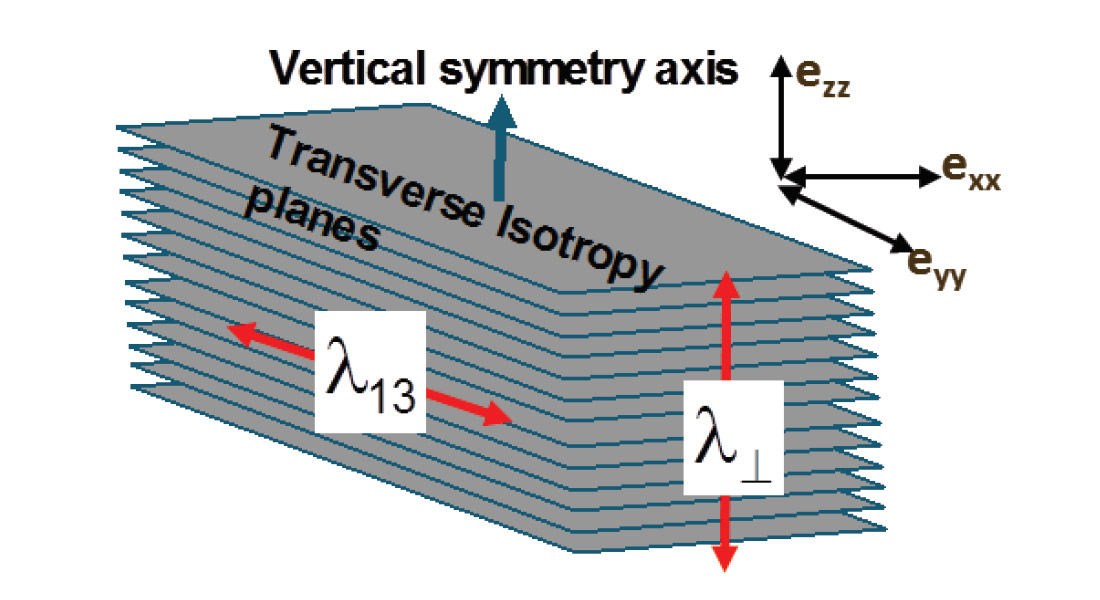
Thomsen initially developed his parameters for TI media with a vertical symmetry axis (VTI as shown in Example 1 above the five term anisotropic VTI stress-strain tensor matrix is considered next by analogy with the isotropic case:

This matrix can be represented in Lamé terms in two ways modified from Sheriff’s Dictionary of Geophysics (1991, page 99).

Case (1) as given by Sheriff:

Where ≡ is measured parallel to layering, ⊥ is perpendicular to layering and * denotes an independent μ*.

Using the c_ijkl to Lamé moduli relations shown in the matrices, From this Thomsen’s δ can be represented as:

and now δ is seen to be a function of the difference between μ* and μ_⊥ in the numerator.

So when μ* = μ_⊥ , δ = 0. Furthermore Thomsen’s gamma γ, that controls shear wave splitting and appears in converted wave AVO as well as Rugers’ AVAZ equation, is therefore represented as:

However, a more common interpretation of shear wave splitting in terms of γ is to consider the numerator in the above equation as the difference in layer parallel μ≡ to layer perpendicular μ denoted as μ_⊥ not μ*. So this VTI symmetry is generally described by only two μ terms related to shear wave phase velocities for vsh waves (polarized in the horizontal plane having Voigt index xy, (Thomsen, 1986) given as:

Consequently if μ* = μ_⊥ then γ is the seen to be the common shear wave splitting expression as a function of μ≡ − μ_⊥ but δ = 0 (Thomsen 1986) as shown above. And for completeness Epsilon ε, the P-wave equivalent to γ, can still be strongly positive and represent the anisotropic P-wave response to VTI media as it is given as:

This is blatantly confusing and is obviously not a realistic representation of VTI anisotropy. As a result there is a more reasonable second possibility for Sheriff’s tensor matrix representation in Lamé moduli terms for VTI media given as:

Case (2):

Where as before ≡ is measured parallel to layering and ⊥ is perpendicular to layering, while λ₁₃ and λ₃₃ are contained in stiffnesses C₁₃ and C₃₃.

So with this version of Sheriff’s matrix Thomsen’s delta δ is represented in Lamé terms as:

These equations reveal δ as being a function of the λ₁₃ − λ₃₃ difference.

By considering a VTI version of Hooke’s law for axial stress in the vertical z-direction given as:

the difference in λ₁₃ and λ₃₃ can be seen as contributing to a difference in axial strain e_zz to transverse strains e_xx e_yy, from Lambda terms only, unlike the isotropic case where the contribution is equal. This suggests that δ is influenced more by variations in Lambda due to both the solid planes and the fluid fill between the planes in the VTI or HTI models shown in Figures 1a, and 1b (Berryman et al 1999).

It is interesting to note that in Thomsen’s DISC 2002 manual he states “…λ does not have a common name, since it is not useful for much in geophysics (despite what you might have heard!).” In the context given here one might also add that if λ is not useful for much in geophysics then neither is δ as it is strongly influenced by λ.

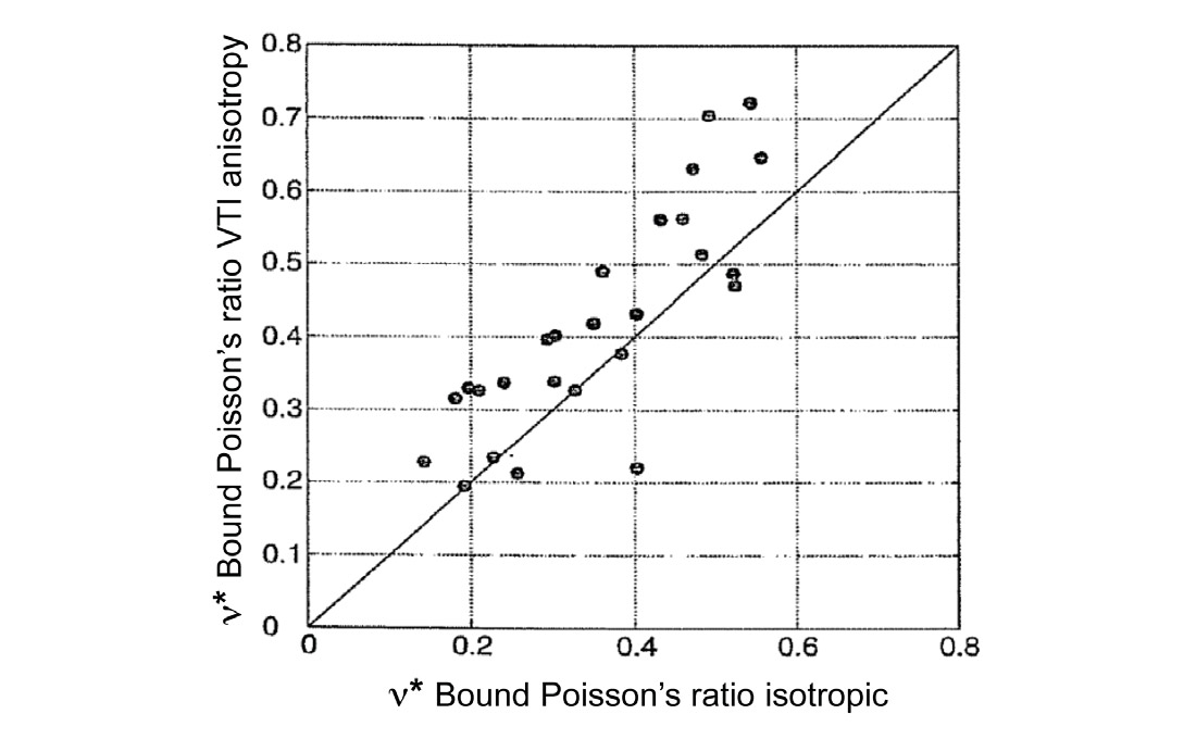
As δ due to VTI is almost always positive (NMO velocity > vertical velocity) so λ₁₃ > λ_⊥ implies stiffer lambda values parallel than across layers shown in the following derivations for the anisotropic VTI bound Poisson’s ratio ν*_VTI from the isotropic form ν* (or CSS):

(From Sayers 2010 SEG DISC notes page 120)

This λ₁₃ > λ_⊥ difference is seen in Figure 5 from Sayers DISC 2010 where ν*_VTI > isotropic ν*

All of the above derivations and matrices were published or shown at various conventions and workshops over a ten year period from 2001 to 2011 by myself and colleagues. Despite this as posted by Evan Bianco of Agile (see above) at the last year’s (2013) SEG convention in Houston Thomsen used the very same matrix in case 2 above to derive his δ in Lamé terms as being a function of the λ₁₃− λ₃₃ or λ₁₃− λ_⊥ difference, as λ₃₃ > λ.

The derivation from Thomsen’s 2013 SEG talk is reproduced here (top line below) and compared to my equivalent that follows from the matrices shown above that were published in the appendices of my article “A tutorial on AVO and Lamé constants for rock parameterization and fluid detection” in RECORDER June 2001.

So from this one can see that Thomsen’s delta differs by a μ_⊥/(λ_⊥+ μ_⊥) term and this leads to a difference in the formulation of the anisotropic VTI bound Poisson’s ratio ν*_VTI that Thomsen presented in his convention paper compared to mine as follows:

When people talk about sweet spot identification in unconventional plays they look for high TOC and more brittle rock. However, high TOC corresponds to higher ductility. It would probably make the determination of the sweet spot more complicated. Would you like to elaborate on this? In the Horn River Basin (HRB), how is Apache trying to characterize the Muskwa/Otter Park units?

Once an inverted 3D volume is obtained from standard AVO SI as described in the workflow of Close et al. (TLE 2012), the rock physics templates described above can be used to construct a rock quality attribute map to predict the stage specific completion’s performance of horizontal well pads. Given the subtle variations in mechanical properties of most unconventional plays, it is difficult to interpret target gas shale zones from the seismic cross-plot alone. However, applying a template enables a plausible geologic interpretation.In fact, to investigate a larger spectrum of possible outcomes, using more than one template allows for a better understanding of variability in production and increases the awareness of uncertainty. As mentioned above, anisotropic models can also be used to interpret the azimuthal AVO attributes to estimate horizontal stress anisotropy and/or fractures.

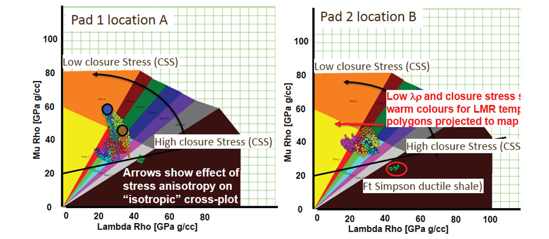
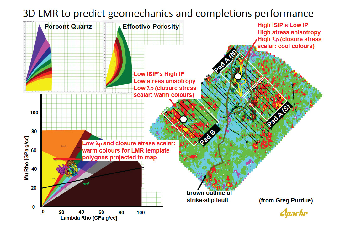
For the Horn River Basin, superimposing seismically derived attributes on templates developed by Perez et al. (2010, 2011) and Goodway et al. (2006, 2010) enables a correlation to be made between λρ, effective porosity and EUR, as seen in the template in Figure 2. Note that a number of seismic LMR cross-plot points extracted along well paths for Pad A, plot to the high end of the λρ range, within the more ductile trendlines. This explains, to first order, the higher ISIP (breakdown pressure) and reduced production from specific stages in the pad. Despite these higher ISIPs, there is a clear relationship between higher EUR and lower λρ, suggesting that this attribute along with the closure stress scalar λ/(λ+2μ) ratio rotation on cross-plots in Figure 2 and 6a) are suitable for mapping optimal production performance in gas shales. This conclusion has been confirmed by the accurate prediction of subsequent completions of Pad B where its resulting initial production is more than double that of the north half of Pad A (Figure 6b).

Acknowledgements

I would like to acknowledge my colleagues at Apache Corporation Marco Perez, Greg Purdue and past colleague Dave Close for their significant contributions to this work. Without their involvement none of this would have been possible.

References

Berryman, J. G., P. A. Berge and Brian P. Bonner, 1999, Role of λ-diagrams in estimating porosity and saturation from seismic velocities, SEG Expanded abstracts, 176-179.

Bianco, E., 2013, Grand Challenges, Anistropy, and Diffractions, www.agilegeoscience.com / Journal/2013/9/30.

Cambois, G., 2000, Can P-wave AVO be quantitative?, The Leading Edge, 19, 1246–1251.

Cambois, G., 2001a, AVO processing: Myths and reality: 71st Annual International Meeting, SEG, Expanded Abstracts, 189-192.

Cambois, G., 2001b, AVO processing: Myths and reality: CSEG RECORDER, 26, no. 3, 30–33.

Castagna, J. P., and S. W. Smith, 1994, Comparison of AVO indicators: A modeling study: Geophysics, 59, 1849–1855.

Close, D., M. Perez, B. Goodway and G. Purdue, 2012, Integrated workflows for shale gas and case study results for the Horn River Basin, British Columbia, Canada, The Leading Edge, 31, 556-569.

Goodway, B., M. Perez, J. Varsek and C. Abaco, 2010, Seismic petrophysics and isotropic-anisotropic AVO methods for unconventional gas exploration, The Leading Edge, 29, 1500-1508.

Goodway W., Chen T., and Downton J., 1997 “Improved AVO fluid detection and lithology discrimination using Lamé parameters; lr, mr and l/m fluid stack from P and S inversions” CSEG National Convention Expanded Abstracts 148-151.

Goodway B., “Practical AVO/LMR: Rock Parameterisation and AVO Fluid Detection Using Lame’ Petrophysical Factors: l, m and lr, mr,” 2002 CSEG DoodleTrain Week Course Notes

Goodway W., 2001 “AVO and Lamé constants for rock parameterization and fluid detection” CSEG RECORDER, June, 2001.

Goodway, B., J. Varsek, and C. Abaco, 2006, Practical applications of P-wave AVO for unconventional gas Resource Plays, Part II: Detection for fracture prone zones with Azimuthal AVO and coherence discontinuity: CSEG RECORDER, 31, no. 4, 52-65.

Hedlin, K., 2000, Pore space modulus and extraction using AVO, SEG Expanded abstract, 1-4.

Perez, M., 2010, Beyond isotropy-Part I: A prestack perspective, CSEG RECORDER, 35, no. 07, 36-41.

Perez, M., 2010, Beyond isotropy-Part II: Physical models in LMR space, CSEG RECORDER, no. 08, 35, 36-43.

Perez, M., D. I. Close, B. Goodway, and G. Purdue, 2011, Developing Templates for Integrating Quantitative

Geophysics and Hydraulic Fracture Completions Data: Part I – Principles and Theory: SEG, Expanded Abstracts, 1794-1798.

Ross, C. P., 2010, AVO ritualization and functionalism (then and now), The Leading Edge, 29, 532-538.

Ruger, A., and Tsvankin, I., 1997 “Using AVO for fracture detection: Analytic basis and practical solutions” TLE, Vol.16, No. 10, 1429–1434

Russell, B. H., K. Hedlin, F.J. Hilterman and L. R. Lines, 2003, Fluid-property discrimination with AVO: A Bio- Gassman perspective, Geophysics, 68, 29-39.

Sheriff, Robert E., 1991, Encyclopedic Dictionary of Geophysics (SEG 1991, page 99).

Sayers, C. M., 2010, Geophysics under stress: Geomechanical Applications of Seismic and Borehole Acoustic Waves, SEG DISC notes.

Thomsen, L., 1986, Weak elastic anisotropy, Geophysics, 51, 1954-1966.

Thomsen, L., 2002 “Understanding Seismic Anisotropy in Exploration and Exploitation” SEG DISC course notes page 1-21

Thomsen, L., 2013 “On the use of isotropic parameters λ, E, ν, K to understand anisotropic shale behavior” SEG Expanded abstracts, 321-324