Why Did I Apply Pre-Stack Interpolation to a Tightly Shot Plains 3-D?

Summary

A 3-D seismic survey was purchased over a channel sand development play that was known to be charged with gas, oil, and water. The 3-D seismic data was of very high quality, and it was initially felt that finding a structurally high location with indications of good reservoir quality would be a trivial matter. As work proceeded, the possibility of unforeseen stratigraphic breaks within the development area became apparent. Initial processing results showed that while there were technically desirable drilling locations, surface constraints such as farm houses, were preventing us from drilling them. The available surface locations were uncomfortably close to character changes in the reservoir that we did not understand. In an effort to understand the character changes being observed, we applied maximum efforts to increase the frequency content of the data. Almost as an afterthought, we applied a pre-stack interpolation process prior to Pre-Stack Migration. We were not surprised to find that the interpolation slightly reduced the amount of random noise in the data. We were, however, shocked at the amount of stability that the interpolation provided to our final high resolution section. This paper primarily illustrates this observation, and secondarily begins to explore these phenomena’s repeatability and ultimate significance to general 3-D seismic.

Introduction: interpretive and drilling problem

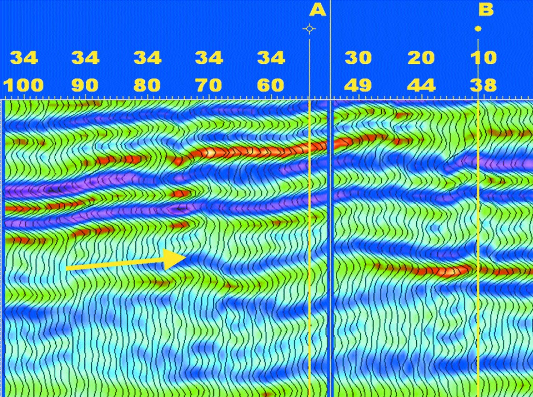
The Cretaceous in Southern Alberta, Canada, where this study focuses, contains a series of fluvial channels, marine sands, and shales. The pool that we develop in this study is contained in a channel sand with thickness up to twenty meters and porosities in the eighteen to twenty percent range. The channel sand can also have abandonment, or tight, facies elements that would serve to separate accumulations of hydrocarbons. Two wells, A and B were drilled into this pool prior to acquisition of the 3D survey. Both wells have thick, porous sands. Well B has a thin oil column over water. Well A is entirely wet. Please see figure 1.

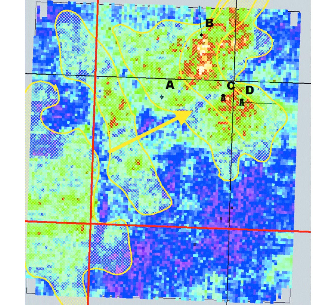
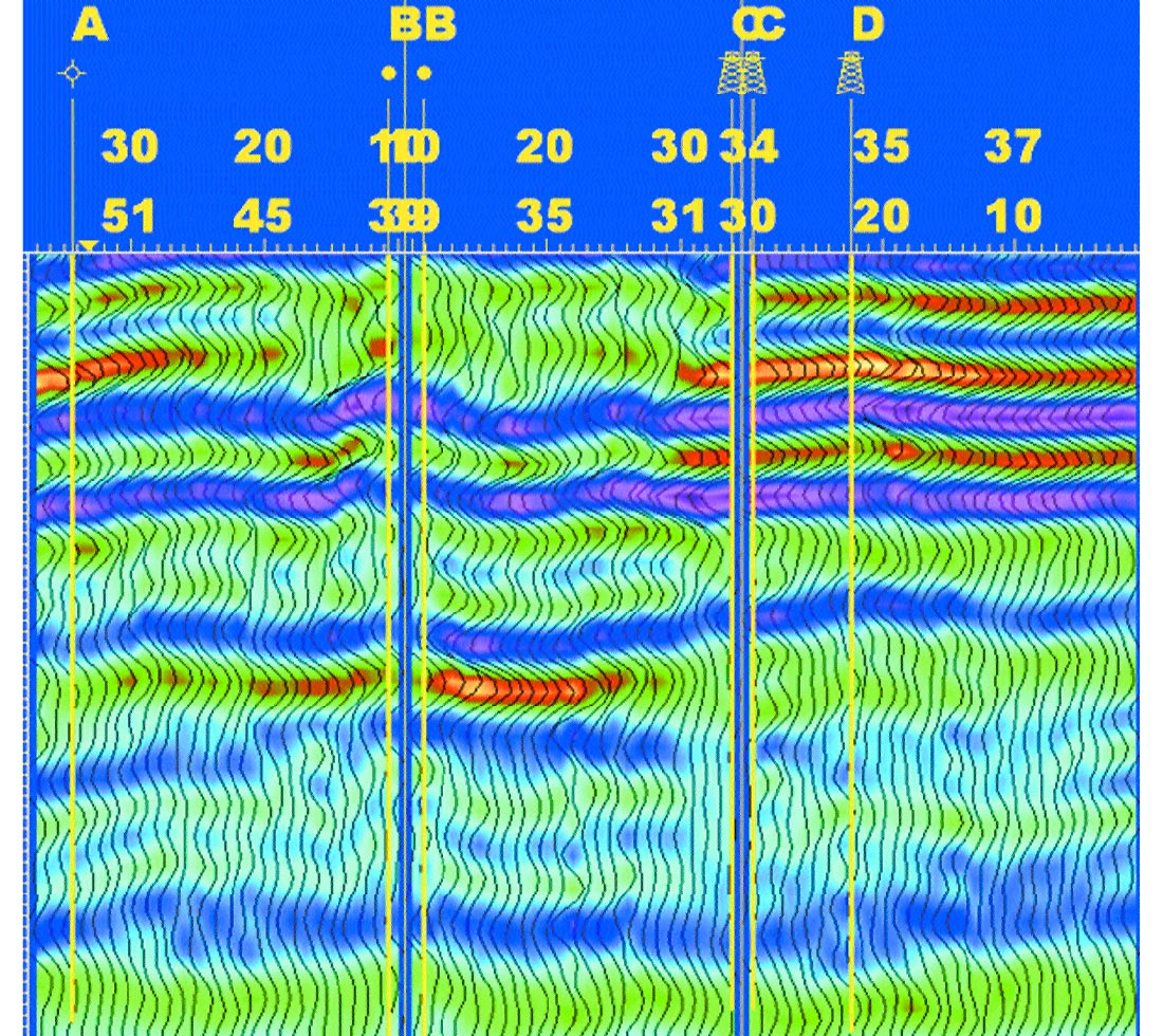
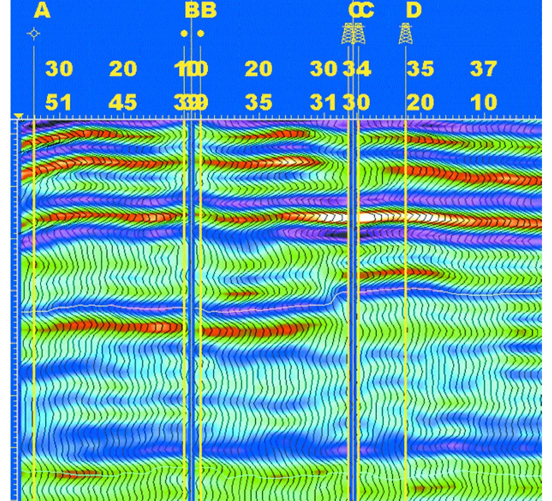
A 3-D was purchased with the purpose of aiding in picking a development location that would have porous sands in the channel, but be structurally higher that wells A and B. The 3-D survey was shot with orthogonal geometry and a tight 280m source and receiver line spacing. The source used was vibroseis, swept up to 110 Hz. Some signal existed at the zone of interest to the upper sweep frequency. The channel zone of interest was imaged as a map-able trough. The initial post stack migration provided a good quality image, wherein the channel trough was mapped. Please refer to the amplitude map of that trough, illustrated in figure 2. Two new well locations are illustrated on the map: locations C and D. Location D is clearly in the heart of the strong trough, while location C is near the edge of a linear feature of lower amplitude. All four locations are shown on an arbitrary line through the 3D, illustrated as figure 3. Figure 3 shows that locations C and D appear higher than A or B, and that both C and D encounter the strong trough event. The weak, linear amplitude feature near location C was of great concern because it was identified as possibly representing tight facies. Location D was clearly the most desirable well to drill next. Unfortunately, surface culture prevented drilling a vertical well there. The nearest vertical possibility was location C.

The debate was on whether we should drill an expensive deviated well to location D, or a cheaper vertical well to location C. If our image was correct to within a bin (30m), location C should encounter the strong trough, or channel, facies. If the image was incorrect by two bins (60m), we would encounter the linear weak amplitude trend. The consequences of a miss-image were not known. The linear low amplitude trend was thought to probably be tighter facies, but we did not know how tight. We hoped to derive a better 3D image and interpretation from the data (and thus break the conundrum of location C versus D) by increasing the resolution and obtaining a pre-stack migration.

Theory: increasing vertical resolution

The data was band limited to 110 Hz by the limited vibroseis sweep and the earth filter, but we still had some ability to shape the amplitude spectrum within that limitation. We chose to follow a familiar and well understood strategy. We would:

• reduce the noise level as much as possible through noise attenuation and stacking
• apply spectral balancing before and after stack
• color correct the data by applying a simple dipole-like filter as per Walden and Hosken (1985)

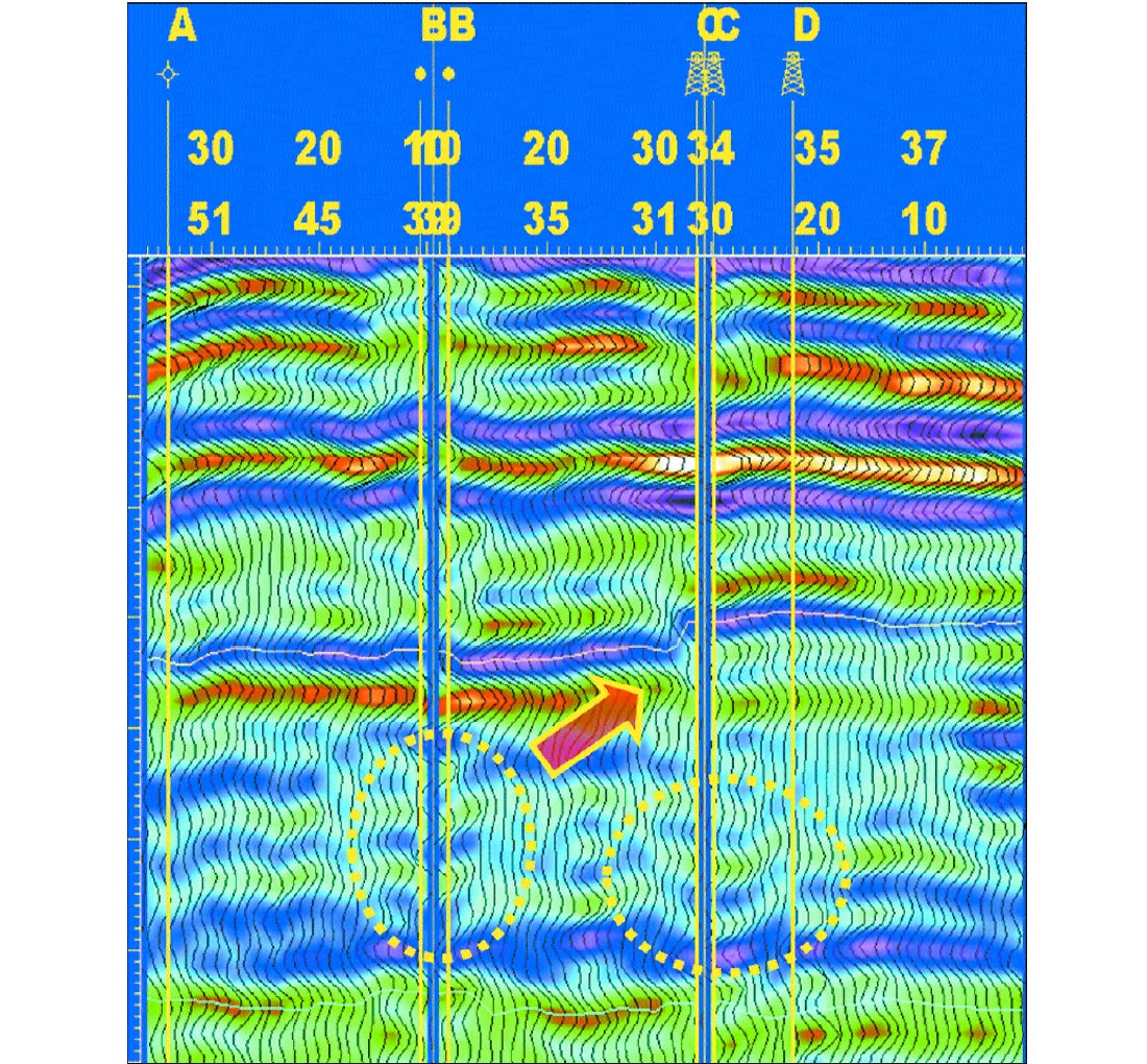
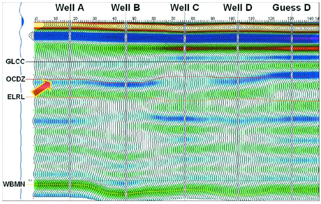
This was applied to data that was also pre-stack migrated. The results were certainly very high frequency, but also very noisy. Please see the new version of the arbitrary line in figure 4. Noisy areas are pointed out with yellow circles. These noise patterns have a shape much like the expected migration operator, leading to the suspicion that some element of the noise pattern is migration noise. The red arrow points out the position of the weak linear amplitude trend noted on the amplitude maps.

Pre-stack interpolation

Pre-stack interpolation is being used more and more as a method of regularization for pre-stack imaging. It is normally being applied in sparsely shot 3-D surveys, and on structural plays. Another application for pre-stack interpolation is to prevent aliasing on large bin 3-D surveys prior to pre-stack migration. The 3D under examination here was tightly shot, with small (30m) bins, and we had little reason other than curiosity to apply interpolation. Nevertheless, we did so, and processed the data using the same high frequency flow as was mentioned above. We were surprised to find that the final results were observably improved. Please see the interpolated version of the arbitrary line in figure 5.

The effect of pre-stack interpolation

In comparing the three versions of the arbitrary line, we can see that the data appears to be much more stable and high resolution with interpolation. The differences appear to be the removal of small arcuate noise patterns that bear a suspicious resemblance to migration operator artifacts. The interpolated line has geologically reasonable, nearly flat events where the standard high frequency result is plagued by these arcuate noise patterns. A possible rationale for this:

• Interpolation for regularization should fill in the holes in the pre-stack geometry, allowing the migration kinematics to work better. That is, less migration artifacts. This 3D survey is tightly shot, with an unusually regular geometry for a land 3D survey. It is interesting that even on this very well shot survey, migration artefacts may be observed on the versions without interpolation.
• At the highest frequency limits of the data, there are numerous breaks caused by low signal fidelity. This accentuates the migration geometry problem by simulating additional “holes” in the wavefield- even on well sampled geometries.
• The interpolation impact on migration is much more apparent at the highest recoverable frequencies, because this is where the migration kinematics are most at jeopardy, both from a geometry and a wavefield fidelity perspective.

In essence, we are saying that the regularizing effect of the interpolation is so remarkable in this case only because we have pushed the frequency content of this data to the limit of its fidelity. This result brings forward the question of whether interpolation should be a standard part of a high frequency flow. Given that the noise being reduced by the addition of the interpolation appears to be largely migration noise, these observations also suggest that interpolation should be considered prior to pre-stack migration generally.

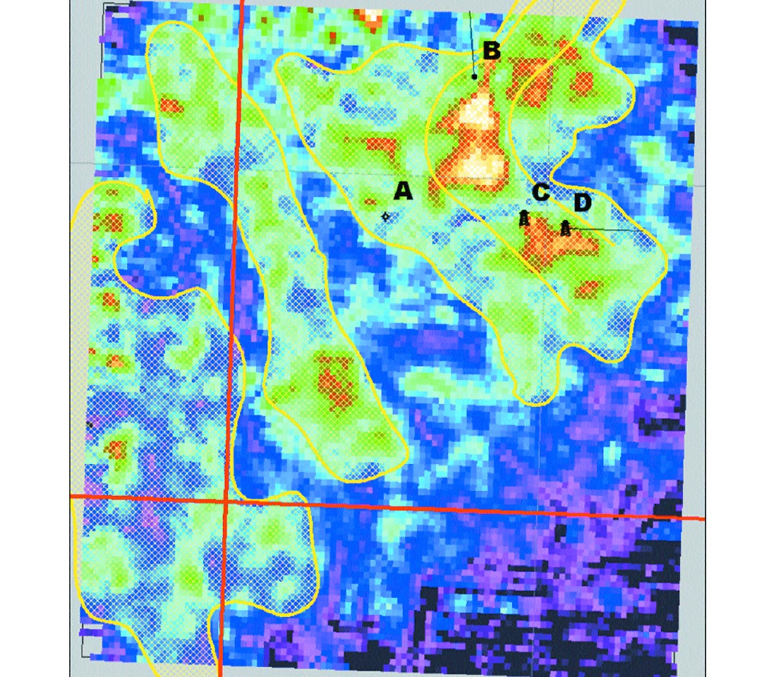
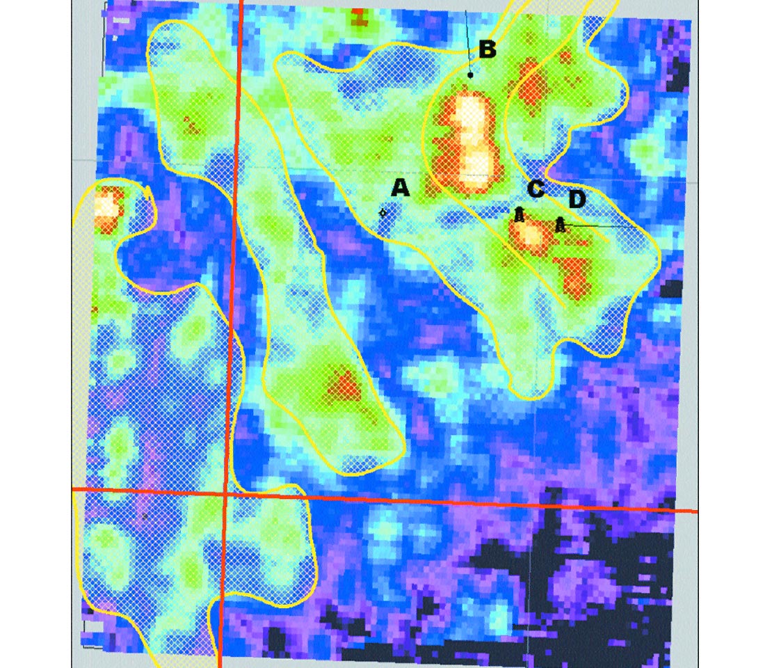
This bold question is yet to be substantiated. Stratigraphic interpretation is also concerned with the fidelity of stratigraphic edges such as the linear low amplitude pattern we observed in figure 2. We may well ask whether that narrow edge is preserved though the interpolation. Figures 6 and 7 compare amplitude maps of the data with the high frequency flow and with the interpolated high frequency flow. Note that both seem to preserve the linear, dim, feature.

Decisions and drilling results

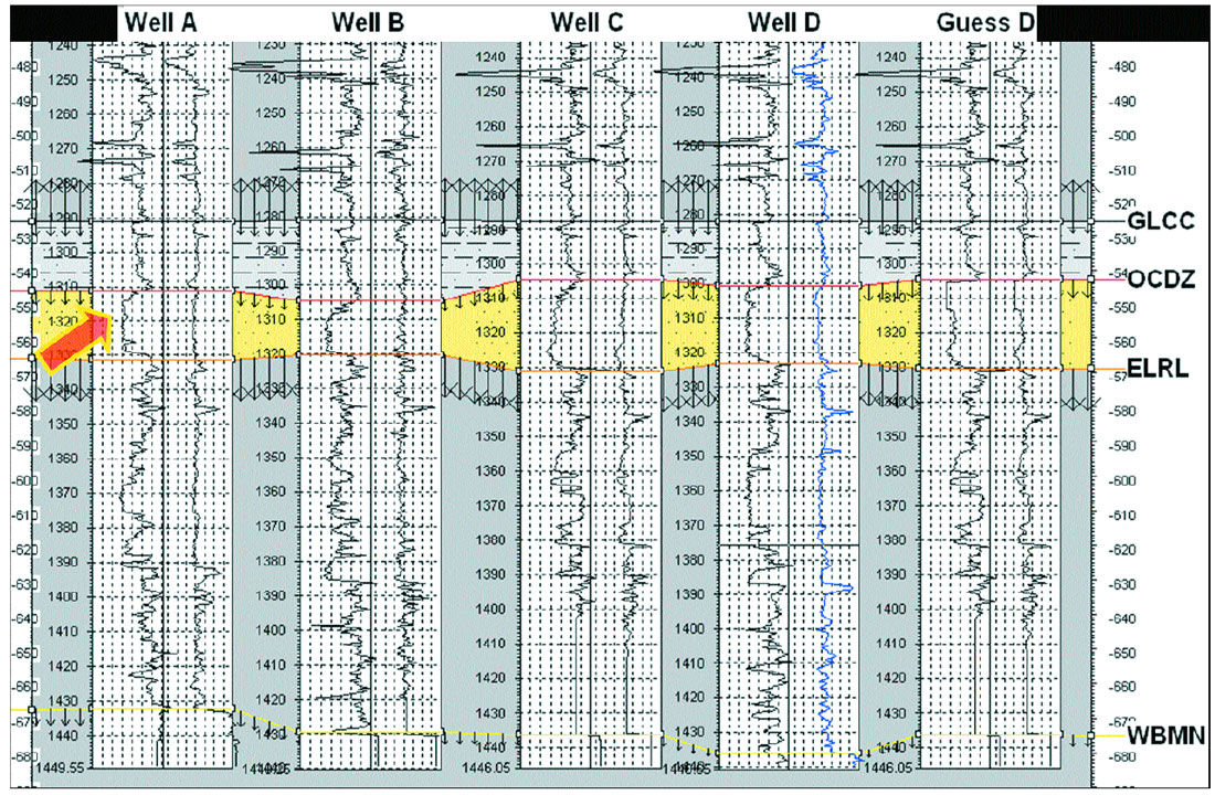
The problem of drilling location C versus D was not resolved by this work. The interpretation remained the same, and location C was still thought to be just within the strong trough event and outside of the dim, linear amplitude event. We decided to drill location C. Location C was found to be a thicker, but somewhat tighter version of the channel we were developing. It had a thicker hydrocarbon column than well A. Modeling with well C suggested that the narrow, linear, dim, feature was in fact rock much like well C encountered: thicker, but tighter sands. Well D was then predicted to be of similar thickness to well C, but with better quality rock at the top of the zone. An actual predicted log was created for well D. Based on this work, well D was drilled, and it came in much as predicted. A model cross section is illustrated in Figure 8 that includes wells A, B, C, D and the predicted well D. The normal incidence synthetic seismic for this model is illustrated in Figure 9. Comparing the synthetic model from Figure 9 to the arbitrary line out of the 3D illustrated in Figures 3, 4, and 5, we can see that the seismic imaged the zone very well. It might be argued that well C ties the character one to two traces away; that of the dim linear trend. This potentially missed image is consistent on all versions of the data, and was not made worse by the interpolation.

Conclusion

Pre-stack interpolation was only attempted on this well sampled plains 3D out of a sense of curiosity. The well sampled nature of the 3D, and its relative lack of structure did not make it an obvious candidate for pre-stack migration or interpolation. Contrary to this lack of expectation the results of the interpolation, combined with an aggressive high frequency flow, produced observably superior results. Our drilling decisions and the results of that drilling were not impacted by this work. Nevertheless, observations from this effort were of use in that they changed how we felt about interpolation and pre-stack migration. We envision that any improvement in the level of noise on pre-stack migrated data may be of advantage in making better seismic predictions. This work puts forward the possibility that pre-stack interpolation applied prior to pre-stack migration may be useful in reducing migration noise on land 3D seismic surveys in general.

Acknowledgements

Thanks to Olympic Seismic, for their kind permission to show the 3D survey at this convention. We also wish to thank Key Seismic, Veritas Seismic, and Sensor Geophysical LTD., for their efforts on the interpolation question.