Using the Scattering Transform to Predict Stratigraphic Units from Well Logs

Applications of machine learning (ML) have become ubiquitous across many domains in both academia and industry. Voice and facial recognition are now robust features in smart phones and cameras, while text learning and behaviour tracking on the internet have created a commodity market for data. Self-driving cars and spatially aware robotics are both machine learning techologies that have received considerable publicity. Recommendation engines on social media, commercial websites, and internet advertisements are everyday examples of the impact of machine learning. ML is helping biologists to progress genomics research (Libbrecht et al., 2015) and help increase the throughput of microscopic cell analysis (Sommer and Gerlich, 2013). Uses of machine learning to aid in medical diagnoses is a particular high-impact field of research (Kononenko, 2001). ML is also impacting geophysics work flows and interpretation software. Russell and Hampson (1997) use machine learning to predict well log properties from seismic attributes and Meldahl et al. (2001) use a neural network to classify gas chimneys in seismic images. Both technologies are available in interpretation software packages, Hampson and Russell and OpendTect respectively.

Geophysicists analyze remote sensing data such as seismic and well logs in order to characterize geological and structural properties. Measurements are visually interpreted for patterns and correlations in order to classify regions that are similar in geological structure. This type of pattern recognition fits well into a supervised learning problem where interpreted data can be used to train a classifier, which can predict interpretations on future data sets. Convolutional neural networks (CNN) have shown success in recognizing patterns in images and signals. Li et al. (2010) used CNN to extract meaningful features from music for automated genre classification and an approach using CNN achieved the best classification results on the competitive MNIST hand writing benchmark (Schmidhuber, 2012). Unfortunately interpretation of the nodes of a neural network is not clear, making it challenging to assign physical meaning to neural network based classifiers. The scattering transform introduced by Andén and Mallat (2014) offers an alternative approach. The scattering transform shares the same structure as a CNN, but the nodes are predefined as multi-scale wavelet transforms instead of being trained. The nodes of the network can directly be interpreted as multiscale measurements of the input signal. Using the scattering transform has achieved competitive classification results on both music (Anden and Mallat, 2011) and image classification problems (Bruna and Mallat, 2013). Of particular interest to problems in geophysics, the multiscale nature of the transform is tied to multifractal signal analysis (Bruna et al., 2015).

The sedimentary layers of the Earth are built up by random depositional processes occuring across different timescales. These multiscale processes form fractal relationships in the strata of the Earth, which is described by the influential work of Mandelbrot (1982). Fractal analysis of well logs by Herrmann (1997) showed that bore hole measurements (well logs) reflect these relationships as multifractal signals. This paper applies machine learning methods in order to classify major stratigraphic units in well log data. The scattering transform is used to extract multiscale features in order to exploit multifractal properties of well logs, and a supervised learning approach was used to train a classifier. This paper briefly describes the supervised learning workflow, gives an introduction to the scattering transform, and presents results of the method applied to gamma ray well logs from the Trenton Black River dataset.

Dataset

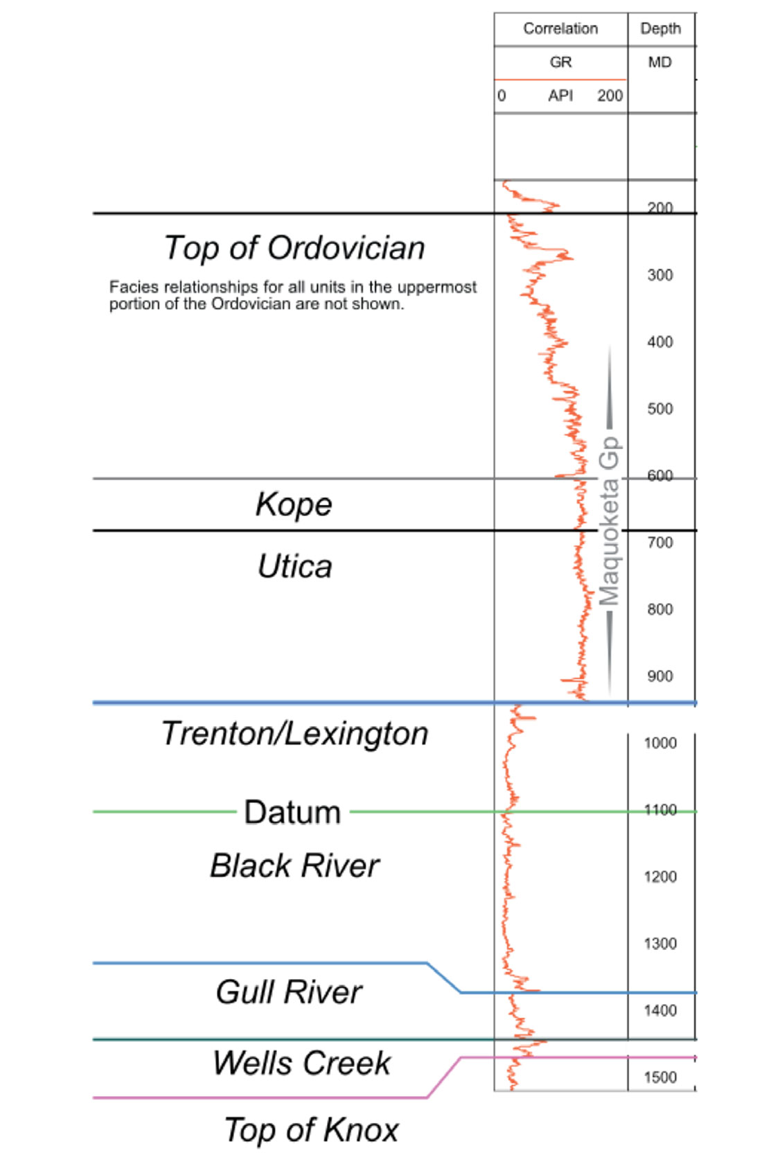
In the early 2000s, the Trenton Black River carbonates experienced renewed interest due to speculation among geologists of potential producing reservoirs. A basin-wide collaboration to study the region resulted in many data products, including well logs with corresponding stratigraphic analysis. The dataset contained 80 gamma-ray logs with corresponding stratigraphic interpretations (labels). Although the region contained more units, some were too thin and pinched out to allow for valid signal analysis. The 5 most prominent units (Black River, Kope, Ordovician, Trenton/Lexington, and Utica) were used for analysis. An example of a labelled log is shown in Figure 1. The dataset can be downloaded at www.wvgs.wvnet.edu/www/tbr.

Methodology

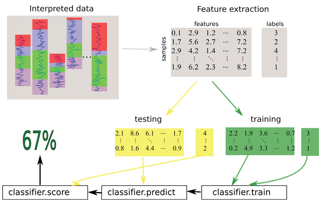
Supervised learning uses labelled datasets to train a classifier in order to make predictions about future data. The general supervised learning workflow is shown in Figure 2. Discriminating raw data samples is often not useful or possible, so the data is first transformed into feature vectors via a feature extraction step. The feature vectors and corresponding labels are used to train a classifier, which aims to find a mapping from feature vectors to labels. This mapping is then used to make label predictions on future unlabelled datasets. The success of a classifier is measured by splitting the labelled data into testing and training sets, where the classifier is trained with the training data and predictions are made on the test data. The predicted labels are compared to the true labels of the test set to measure the success of the training.

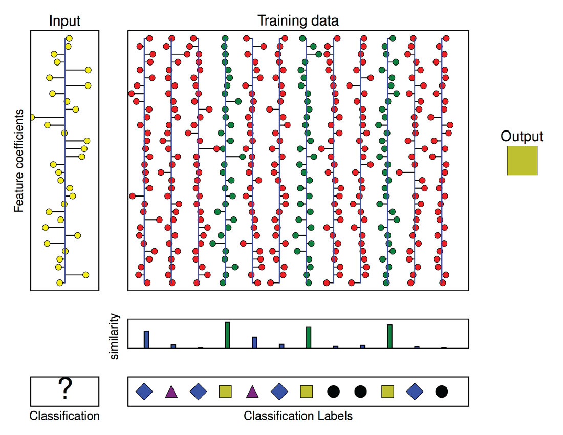
This study used the scattering transform to extract features from gamma ray logs to feed a K-Nearest Neighbours (KNN) classifier. The KNN classifier measures the Euclidean distance between all vectors in the training set and the mode of the labels of the K closest vectors is chosen as the predicted label (Figure 3).

Scattering transform

At a very high level, a wavelet transform ψ_λ uses a bandpass filter bank λ to decompose a signal x[n] into J signal bands. Analogous to the Fourier transform which decomposes a signal into frequencies, the wavelet transform is considered to be a decomposition into scales. The scattering transform exploits multiscale relationships in sig nals using a cascade of wavelet transforms, magnitude, and averaging operations. Figure 4 shows the action of one scattering transform window on a signal.

At the zero-level of the transform, the S₀ output coefficients are simply x[n] averaged by a window ϕ–i.e.,

The first layer of the network is formed by taking the magnitude of the wavelet transform ψλ1 of x[n] and the S1 output coefficients are then generated by averaging along each scale in the filter bank λ1 by the window ϕ–i.e.,

Referring to Figure 4, each win tput coefficients, where J is the number of scales in λ₁.

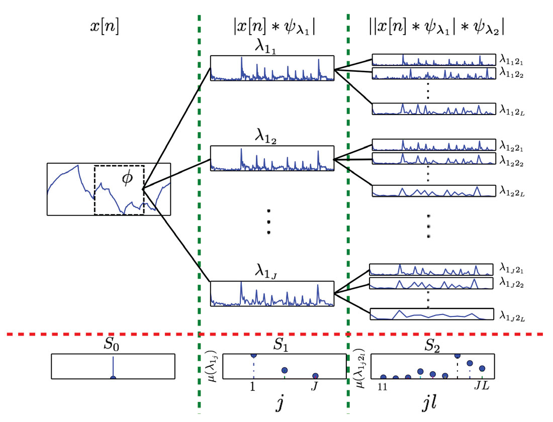
The second layer of the transform is realized by taking the magnitude of a second wavelet transform ψ_λ2 of each signal in the first layer of the network. Averaging is performed to make the S₂ output coefficients – i.e.,

Again referring to Figure 4, the S₂ output contains JL coefficients where J and L are the number of scales in λ₁ and λ₂. Note that the second layer contains multiscale mixing coefficients λ1j 2l . The notation λ_1j2l refers to lth scale of λ₂ operating on the jth scale of λ₁.

This process is repeated to a defined network depth of m – i.e.,

This study used a two-layer network, as the number of coefficients becomes unmanageable for deep networks (large m) and Bruna and Mallat (2013) found only marginal classification improvement for m > 2. Dyadic wavelet banks of Morlet wavelets were chosen for ψ_λm and 256 samples was found as the best choice of averaging window size. The scattering transform was applied to gamma ray logs to form feature vectors from the S₀,S₁, and S₂ coefficients. The opensource MATLAB implementation ScatNet was used for calculating the scattering transforms.

Results

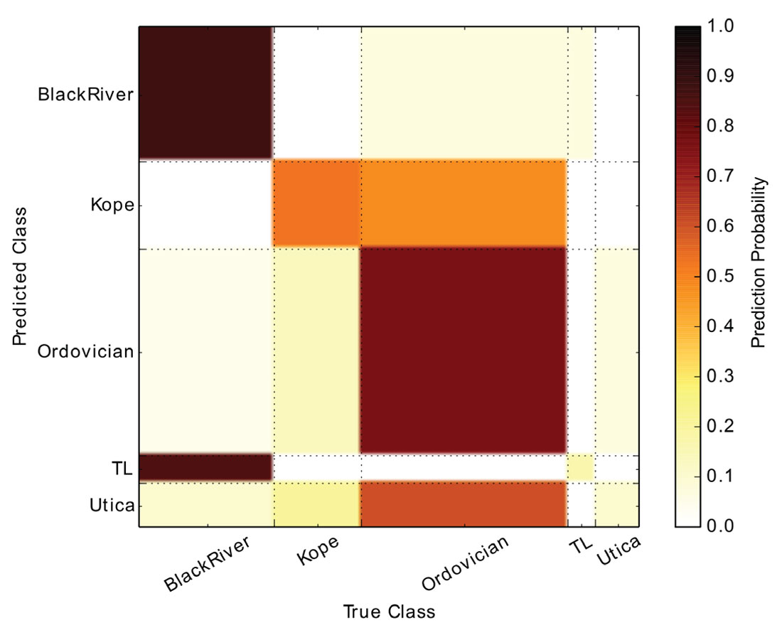
The classifier had an overall prediction rate of 65%. The confusion matrix (Figure 5) shows the prediction and misclassification rates for each unit type. The thicker units, which inherently contained more data samples, showed the best performance. This is expected, as having more training data for a particular label increases the chances of having similar vectors and better matches in the KNN classifier. The two thickest units, Black River and Ordovician, had the best prediction rates. Figure 1 and Figure 5 show that sequential units in the stratigraphic record were the most likely to be misclassified as each other, for example Trenton, Lexington, and Black River. These units may actually come from the same or similar depositional systems and would share similar multiscale structure in the well logs. More detailed assessment of the geology and the method used to interpret stratigraphy is required in order to better understand these results.

Discussion

Assessing the results in a quantitative matter is highly uncertain, as the labels in the “truth” data set are inherently subjective. The work of Bond (2015), as well as recent work by Hall et al. (2015) has shown significant deviations of interpretations on the same section of data. Additionally, what a geologist interprets as a stratigraphic unit can be somewhat arbitrary, and may be based on subjective information other than textural patterns in the data.

The scattering transform is highly parameterized and results would likely be sensitive to choices of wavelet banks and window sizes at each level of the transform. This basic study used dyadic Morlet wavelets at each level in the transform and through experimentation found 256 samples as the best choice of window size. Experiments using wavelet transforms with higher vanishing moments would be beneficial, as more vanishing moments can result in a sparser representation. Sparse feature vectors are generally easier to discriminate. Using different wavelet transforms at each level could also have impact; however, these types of parameter tuning approaches require cross-validation studies on larger datasets.

Due to availability of data, this study was limited to the gamma ray log and did not make use of any a priori knowledge of the region. Incorporating additional log measurements (i.e. sonic, resistivity, etc) would help corroborate the classification, as stratigraphic tops can be interpreted on many different log measurements. A priori information such as stratigraphic ordering and thickness are reasonable assumptions Ben Bougher Continued on Page 32 that should be incorporated as features or penalties in the classification problem in order to boost classification accuracy.

There is a strong correlation between number of samples and classification accuracy, which indicates the need for more data. Generally, training a classifier requires many samples of labelled data. The availability of open labelled datasets for research have proved to be a valuable resource in many other fields. The TIMIT dataset exists for acoustic-phonetic voice classification and GTZAN dataset supports machine learning for music genre classification. The MNIST digit recognition dataset a provides a popular benchmark for hand-written digit recognition, while the CURET and OUTEX sets provides labelled data for image texture classification. Kaggle is a popular website where datasets from many industries are made available as open machine learning competitions. The sensitive nature of interpreted geophysical data makes public datasets in geophysics extremely scarce, but without useful data it is difficult to realize the same ML progress experienced in other fields.

Conclusion

Machine learning takes time and data in order to be effective. This paper used supervised machine learning to predict stratigraphic interpretations from well logs with moderate success (65%) on a relatively small set of data. The scattering transform was used to extract multiscale features from gamma ray logs and a KNN classifier was used to make predictions. Continued research on larger datasets is required to fully assess the usefulness of the approach.