Using Advanced Seismic Imaging Tools to See the Invisible Beneath Foothills Structures

Introduction: the imaging problems

Oil and gas exploration in the Foothills of Western Canada is a mammoth industrial endeavor. Members of major Canadian and international oil and gas companies rub shoulders with their counterparts in smaller companies and with individuals and companies who develop exploration prospects, acquire and process geological and geophysical data, drill exploration wells, and bring the hydrocarbons to market.

The seismic industry is but a small part of the entire exploration picture, and the seismic imaging “cottage industry” is but a small part of the seismic industry. Still, the role of seismic imaging is central to the Foothills exploration effort. The structural contortions of Foothills geology and the highly variable quality of Foothills seismic data combine to produce huge risks in drilling into any structural target. The exploration community relies on seismic processing (imaging in particular), perhaps more than any other single link in the exploration chain, to reduce those risks. Stepout exploration, moving along trend from one structure to the next, requires seismic images to map the new structure and its relationship to the first. At the other end of the exploration spectrum, rank wildcat exploration, sometimes hundreds of kilometers from the nearest existing well, relies almost entirely on seismic imaging in one form or another, plus “trendology,” to determine whether there is a subsurface structure worth drilling.

On the other hand, seismic imaging is highly constrained, both by the quality of the seismic data and by the cost of the imaging product. We mention a few of the data quality issues that affect Foothills seismic imaging. Irregularities in near-surface structure and velocity, inadequate penetration of energy from seismic sources, poor geophone coupling on surface carbonate rocks, surface scattering of energy from the sources, and other effects, all combine to reduce the signal on seismic records. Large velocity contrasts cause uneven focusing of seismic energy in the subsurface, making the complex geologic structures associated with the velocity contrasts harder to image. Reflecting horizons appear suddenly on seismic records, then disappear just as suddenly, leaving holes that might be interpreted as the effects of large-scale faulting and folding, or might merely represent no-data zones.

In addition to data quality problems caused by the geology itself are the problems caused by the economics of some Foothills plays. It makes no economic sense to spend more money on acquiring and processing seismic data than a prospect can pay out in a reasonable time. As a result, seismic acquisition is often less than ideal for imaging the subsurface. For example, 2D and 3D programs are often acquired with a particular objective horizon in mind and with little or no flexibility in the horizon’s location. If that horizon is not where the designer thinks it is, there might not be adequate aperture to record all the diffracted energy from the horizon. As a further example, 3D Foothills data are necessarily sparser than is desirable from an imaging point of view. The large separation of source lines and receiver lines in a 3D cross-spread experiment makes it hard for a migration program to obey wavefield sampling theory while moving energy from one line to the next. Sparse 3D data also make sparse statistics for calculating static corrections and near-surface velocities.

Given these problems, modern seismic imaging techniques perform remarkably well, especially with the help of techniques that are used to apply some estimation or prior knowledge of subsurface parameters such as velocity. These techniques are especially helpful when they can be driven in an intuitive way by an interpreter or a processor who has some knowledge of the structural style and the subsurface velocity. For most plays, in fact, the most serious imaging problems are due to data quality issues or poor knowledge of velocity, and not to the imaging algorithms.

In this article, we combine a description of some of the advanced techniques that have been successful in imaging structures beneath complex Foothills overburden, with a case history from the Blackstone area of Alberta illustrating their use. These advanced techniques allow us to perform anisotropic prestack depth migration and velocity estimation efficiently in an interpretive fashion, producing both a final depth image and a geologically plausible velocity model. In the case history, we contrast a processing flow that uses these tools with more standard poststack and prestack time migration flows.

Some advanced imaging solutions

Using seismic modeling to validate our depth migration routines

We begin our list of advanced imaging technologies with one not normally considered to be an imaging technology: seismic modeling.

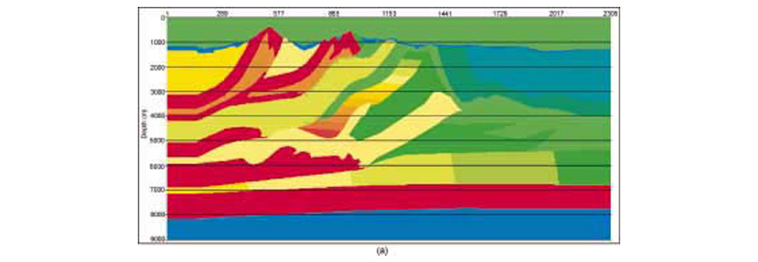
We know that our depth migration programs work well in imaging complex Foothills structures, at least when we have a good idea of the seismic velocities. How do we know that? Because we’ve tested them against some very tough synthetic model seismic data. Figure 1(a) shows a velocity model based on southern Alberta geology, and Figure 1(b) shows a prestack depth migrated (PSDM) image from finite-difference data acquired along this line. The model data contain all the effects of acoustic wave propagation, including multiples, head waves, etc. The Kirchhoff migration program has successfully imaged these data, except for a break along the basement directly below the steeply dipping carbonate thrust sheet that outcrops at the highest elevation. In particular, the target bumps near 6000 m below datum are very well imaged. This model shows the imaging capabilities, as well as the limitations, of the migration program. Migrations of other finite-difference synthetic data sets, from models with greater structural complexity than the present model, have produced images of quality comparable to this one. Given these results, and despite the fact that we never have perfect velocities for migration, we conclude that Kirchhoff depth migration is up to the structural imaging challenges presented by most Foothills data. The imaging cottage industry is moving forward, however, and in the not-very-distant future will be able to offer even more accurate depth migration techniques, such as finite-difference migration.

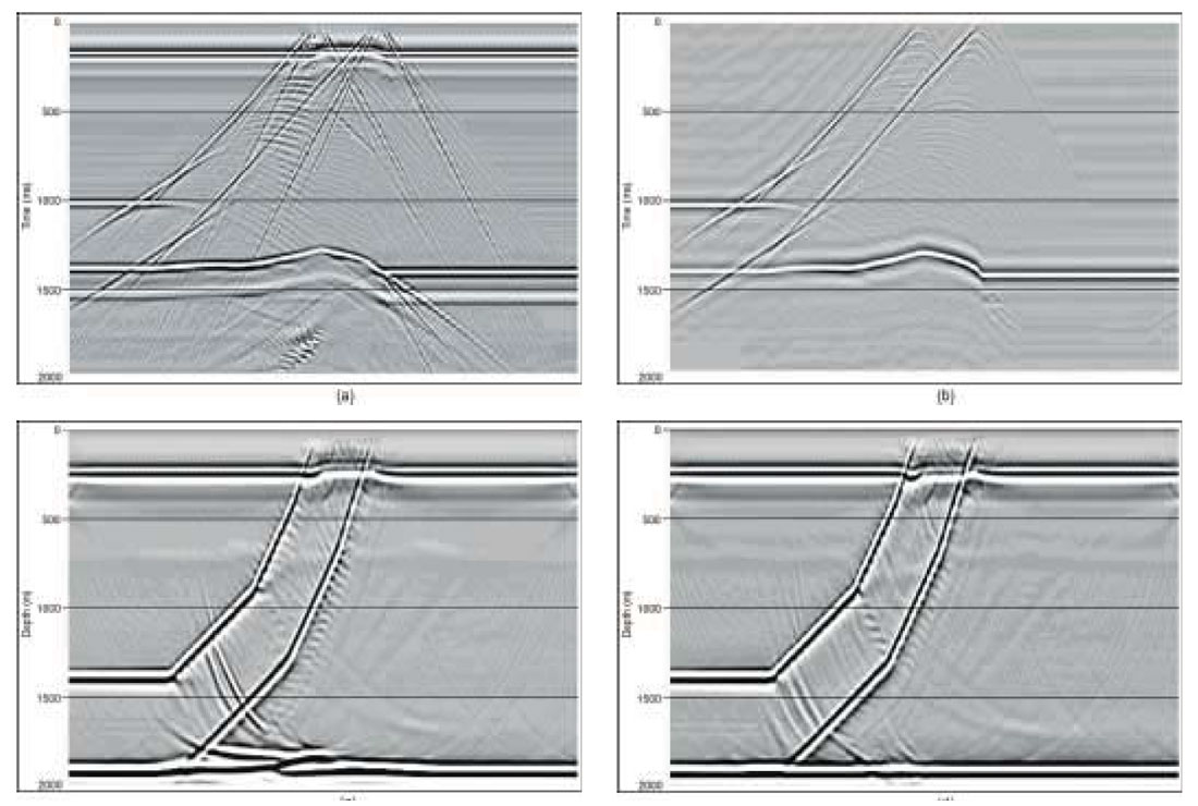
Numerical modeling and physical modeling are useful for testing our imaging algorithms for structural imaging fidelity, amplitude fidelity, steep-dip capability, and so on. They are also useful in helping with survey design, and in testing geologic hypotheses, e.g. can such a geologic structure produce the seismic response that we observe? In the latter application, it is important that the modeling be efficient, for we might want to test a number of geologic scenarios. As valuable as finite-difference and physical modeling are, they are not efficient. So it is useful to have other seismic modeling capabilities in our arsenal, and it is natural to turn a well-calibrated Kirchhoff migration program into a modeling program. (But not for the purpose of testing the original Kirchhoff migration program!) In Figure 2, we show an example of elastic finite-difference modeling (vertical component) and acoustic, anisotropic Kirchhoff modeling on a thrust model, as well as isotropic and anisotropic Kirchhoff prestack migrations of the finite-difference data. The modeled records are zero-offset records, and the migrations are stacks of all the migrated offsets. This model was originally acquired as a physical model (Leslie and Lawton, 1998) to illustrate the problems that arise when we produce seismic images beneath dipping thrust sheets without considering the effects of seismic anisotropy. The match between the finite-difference and Kirchhoff records is excellent, validating the anisotropic raytracer used in the Kirchhoff modeling and migration codes. Some of the minor differences in the records can be ascribed to mode conversions present on the finite-difference record but absent from the Kirchhoff record. Others can be used to explain the artifacts present on the Kirchhoff migration of the finite-difference data.

Turning-wave tomography for near-surface model building

Determining near-surface velocity structures is a crucial first step in seismic data processing and depth imaging. An inadequate near-surface velocity model will result in incorrect statics corrections for time domain processing. For depth migration, even a modest inaccuracy in the near-surface velocity model can introduce large errors in both raypath and traveltime calculation, and can significantly deteriorate the seismic image at depth, especially in the areas with large lateral velocity variations.

Many refraction methods have been developed over the years for near-surface velocity determination, primarily for the purpose of statics solutions. Refraction methods are appealing because the shallowest portion of a seismic record is often dominated by source-generated noise, and accurate identification of reflections is difficult. The first arrivals, on the other hand, can be clearly identified and often represent the best data available for near-surface velocity estimation. Traditional refraction methods assume that the near-surface velocity structure can be represented by a layered model and that first arrivals can be treated as refractions from the model’s interfaces. As a result, these methods cannot model velocity inversions or vertical gradients within each layer, and may fail to accommodate strong lateral velocity variations. By treating first arrivals as refractions, they are also unable to determine the first layer velocity v0. This results in a trade-off between interface depths and layer velocities in a derived velocity model, making the model inadequate for imaging processes such as depth migration which are more sensitive to local velocity variations than is the statics solution.

An inversion method for the accurate determination of near-surface velocity structures has been introduced by Zhu and Cheadle (2000, 2001). The velocity structure is represented by a grid model. Each node of the grid is assigned a velocity and the node velocities can vary in an arbitrary fashion capable of representing strong velocity variations in both vertical and horizontal directions. Also, first arrivals are now treated as direct body waves propagating along turning rays, enabling the method to determine the first layer velocity as well.

The node velocities are determined by solving a nonlinear least-squares problem which minimizes the differences between the observed traveltimes of first arrivals and those predicted from the grid model. The nonlinear inverse problem is reduced to solving iteratively a regularized, linear least-squares problem using the LSQR algorithm introduced by Paige and Saunders (1982). The inversion is regularized by including in its matrix equation both smoothing and stepsize constraints; the former reduces the roughness of the velocity model and the latter limits the linear approximation within a trust region during each iteration.

As the inversion requires intensive raytracing, an accurate and efficient algorithm for traveltime and turning raypath calculation is essential for practical applications. The algorithm must also be robust and devoid of the shadow-zone problem which has hindered tomographic methods based on traditional raytracing techniques. We recently developed the grid raytracing (GRT) technique (Zhu and Cheadle, 1999) specifically for this application. This method calculates traveltimes and wave propagation vectors by tracing rays locally within a grid cell, and has been shown to be highly accurate and efficient in modeling turning rays in near-surface environments. Other traveltime modeling techniques such as wavefront construction and the fast marching algorithm can also model turning rays without shadow zone problems. Tests show that GRT is about two orders of magnitude more accurate than the fast marching method and up to eight times faster than wavefront construction. These attributes make GRT ideal for an iterative inversion for complex near-surface velocities.

Model example of near-surface model building

We investigated effects of near-surface velocity estimation on depth migration using the 2D Canadian Foothills finite-difference model data set of Figure 1. The uppermost 1400 m section of this model is shown in Figure 3(a). The entire model is about 32.6 km long and 10 km deep, and is characterized by large lateral variations in both velocity and topography. First arrivals were picked from the synthetic data to a maximum offset of 3600 m. We first estimated the velocity with a conventional refraction method and smoothed with a 100 m Hanning window in both vertical and horizontal directions. The resulting velocity model is displayed in Figure 3(b). We used the smoothed model as an initial model for the tomographic inversion described in the previous section. The grid model consists of 1305 x 56 cells with a grid spacing of 25 m in both vertical and horizontal directions. The final velocity model shown in Figure 3(c) was obtained after five iterations of tomographic calculation. A comparison of Figure 3(a) and 3(c) shows a close agreement between the true and inverted velocity models, even in some small details, indicating that the tomographic method is capable of recovering near-surface velocity structure in geologically complex areas.

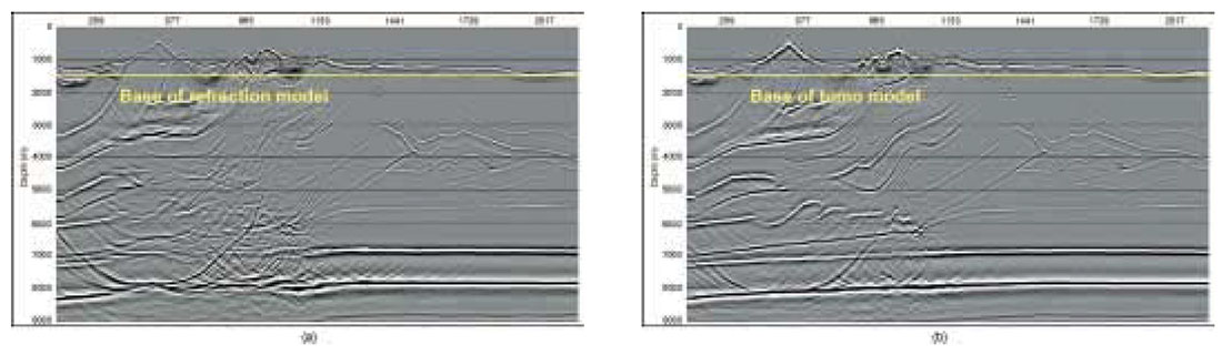
To demonstrate the effects of the near-surface velocity model on prestack depth migration (PSDM) of the synthetic data, we constructed two velocity models by merging the near-surface models from Figures 3(b) and 3(c) respectively with the exact velocity model at 1400 m depth below highest elevation. Figure 1(b) shows the PSDM section obtained with the exact velocity model while Figures 4(a) and 4(b) display respectively the sections produced by the models constructed with the near-surface models from Figures 3(b) and 3(c). The results clearly show that inaccuracy in a near-surface velocity model can severely deteriorate the seismic image at depth and make the process of determining the deeper portions of the velocity model more difficult. The near-surface velocity model determined by the tomographic inversion method has significantly improved the depth imaging, and increases the potential for deriving the deeper model by conventional reflection analysis techniques.

Turning-ray tomography is a general procedure for near-surface model building, providing both static corrections and near-surface velocities as inputs into prestack migration. For PSDM, we can choose to use either the static corrections or the velocities, but for prestack time migration (PSTM), we simply apply the static corrections to the seismic data. Our approach to PSDM uses the velocities to provide the uppermost layer of the velocity/depth model for migration. In theory, this is more correct than applying static corrections to the seismic data, but in practice it carries a certain risk. This is the risk that the rapid variation between the low velocities in the near surface and the much higher velocities just below the near surface will cause problems with the depth migration program. Extensive experimentation (some of it on model data) has shown this not to be the case: the raytracers used in both the tomographic inversion and the Kirchhoff migration program are extremely robust.

Prestack depth migration versus prestack time migration

Between the standard flow culminating in poststack time migration and the advanced PSDM flow lies PSTM, which represents a compromise between processing speed and interpretational resolution. In this flow, we perform the prestack time migration as a series of constant-velocity migrations, providing a cube of migrated stacks from which we can select spatially-varying imaging velocities by picking the velocity panel with the best-focused image at each location. (In 3D, we do this analysis along closely-spaced target lines.) In doing this, we use criteria such as stack power and optimal diffraction collapse to guide our picking of the PSTM velocity field. We then use the final velocity field to perform a final full volume migration. We have already mentioned that our advanced flow is interpretive, and we must also emphasize the interpretive nature of standard velocity picking for PSTM, at least for Foothills data. It is important for the seismic processor who actually does the PSTM to be aware of the structural style and seismic velocities of the area in order to discriminate between conflicting but plausible structures. In practice, these decisions are left to the processor with varying amounts of guidance from the interpreter.

The standard method for depth migrating Foothills data is Kirchhoff migration. As we mentioned earlier, we have tested our depth migration programs extensively on synthetic model data in order to optimize both accuracy and speed. Recently, migration methods with greater theoretical accuracy, such as finite-difference migration, have become available, and these will soon be competitive economically with Kirchhoff migration. Many details need to be worked out, however, before these methods can be used for production processing. Technical issues with these methods include their ability to migrate accurately from topography and to produce common image gathers that can be analyzed for velocity updating. The greatest barrier to their use, though, will be their need for regular spatially sampled data, which can be accomplished today only at great expense, during either acquisition or preprocessing.

Interactive reflection tomography

In our PSDM flow, we perform a number of PSDM iterations. To perform our first iteration, we place the tomographically inverted near-surface velocities atop a smoothly varying initial velocity/depth model. For the Blackstone data set discussed below, the inverted velocities are shown in the upper 500m to 650 m of Figure 5(a). These velocities, computed without assuming a layered model and without constraining the inversion, are certainly plausible. Velocities along the floating datum marking the base of the near-surface correspond well with the expected formation velocities in the initial model. It is common practice to use an initial model based on a Dix inversion of the imaging velocities used for time migration. For areas as structurally complex as the Foothills, however, we find that equating the imaging velocities used in time migration with RMS velocities can lead to significant errors in PSDM. Instead, our initial model might be a heavily smoothed version of what we initially believe the structural model to be (more interpretation!), or it might even be a single function picked from a nearby well log.

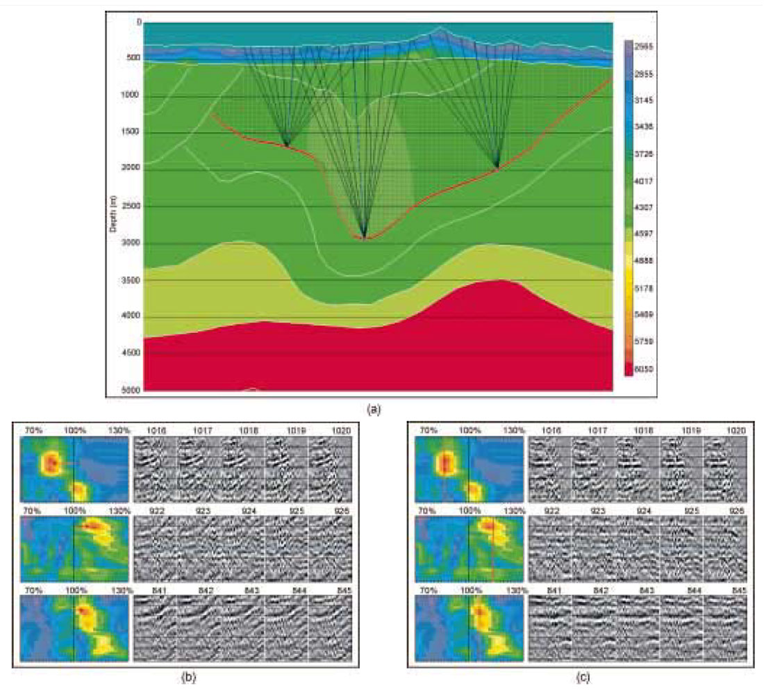
Velocity model updates for subsequent iterations are performed using an interactive reflection tomography tool (Gray et al., 2000). This tool represents the velocity as a gridded model between horizons that separate major geologic units. Proceeding from the top down, we update the velocity in one or more of these units before we repeat the migration. At selected locations, we use raypaths shot upwards from the base of a target geologic unit (Figure 5(a)). Velocities in overlying layers remain fixed at values determined from previous iterations. The effects of a velocity change along the ray segments within the active unit are computed and registered on the displayed depth-migrated image gathers (Figure 5(b) and 5(c)). The crucial feature of this tool is its interactive nature. Applying a percentage velocity change within a unit produces an immediate change in the moveout on the image gather. The velocity change might make the gather more flat (a good thing), it might make it smile or frown (a bad thing - velocity too slow or too fast), or it might even destroy the continuity of the event. Many different velocities may be tried, and most of them rejected, in just a few seconds, before the velocity that flattens the gather is accepted. Many different locations can be scanned quickly to determine where the data quality best supports the velocity analysis.

Alternatively, we might investigate - again, interactively - the effects of the velocity changes on the stacks in the vicinity of the active horizon, with the various stacks computed using the moveout dictated by the various velocities. The stack power along the horizon can also be calculated over the range of trial velocities and displayed below the data stacks. Velocity picks can be made on any of the various displays. These interactive features allow us to investigate efficiently the effects of many different velocity functions within a geologic unit, giving us a very quick preview of the results of remigrating the data. We can use it to investigate many geologic hypotheses quickly, without the expense of many migration iterations. Once we discard the least likely of these, judging from either the seismic data or the geologic constraints, or both, we can focus on the most likely model, fine-tuning the velocities to optimize the image.

Anisotropic depth migration

In Figures 2(c) and 2(d) we showed the effects of ignoring anisotropy when performing PSDM on a simplified Foothills structure. In this example, ignoring anisotropy caused false structure on the image. This false structural high makes a tempting drilling target. Anisotropy can also cause lateral mispositioning (Vestrum et al., 1999), and has been blamed for many a Foothills well trajectory missing the apex of its anticlinal target. Many Foothills areas are known to contain dipping shale-dominated clastics, which are typically anisotropic. Including anisotropy in PSDM requires us both to estimate anisotropy parameters and to incorporate them into the traveltime calculations for migration.

We parametrize the anisotropy using the Thomsen parameters and , which, when combined with the “slow” velocity and the dip angle of the symmetry axis (both typically measured normal to bedding) are incorporated into ray equations that provide migration traveltimes as well as raypaths and traveltimes for interactive tomography. In our interactive tomography procedure, the image gathers or stacks can be scanned as a function of the anisotropy parameters and just as they can be scanned as a function of velocity. In fact, they can be scanned in combination with each other or in combination with the background “slow” velocity perpendicular to the anisotropy axis. Doing this allows us to pick the optimal of velocity, and that best flattens the image gathers or best focuses the stack. If VSP data are available, traveltime inversion of first arrivals from updip and downdip directions may also be used to estimate the Thomsen parameters directly (Kirtland Grech et al, 2001). We then typically check our estimates from either of these methods by running a suite of PSDM images over a limited range of anisotropy parameter values to confirm that the chosen values produce the optimal image.

3D

Anyone who has driven through the Foothills can appreciate the 3D nature of geology, at least near the Earth’s surface. On the other hand, a great deal of Foothills exploration continues to be 2D. While it is true that there is considerable 3D variation in fold-belt structures on the scale of a seismic wavelength, many, if not most, of our structural targets have a dominant dip direction, with only gentle variation along strike. As exploration gradually becomes development, 2D is gradually giving way to 3D, and our advanced seismic imaging tools are being used more and more in 3D.

A case history from Blackstone, Alberta: standard versus advanced processing

In this section, we apply the advanced techniques presented above to the problem of imaging several thrust sheets beneath complex Foothills geology. To set the stage for this, we first described more standard (time) imaging technology applied to the same area. For this 2D data set, the combination of complex overburden and subtle imaging targets provided insurmountable problems for the standard flows. This is by no means a universal phenomenon – we often observe images from PSTM that are similar to, or even better (i.e., clearer) than, our best PSDM images. Even when this happens, though, we typically have greater confidence in the target locations on the PSDM images, especially when we have accounted for anisotropy.

The standard poststack flow is straightforward. Its goal is to produce a final stack that can be migrated quickly using a highquality finite-difference time migration program. First, refraction and residual static corrections are applied to the data (all from surface), in combination with two or more iterations of velocity analysis. Next, the data are NMO- or DMOcorrected and stacked, then referenced to a flat datum using elevation static corrections to prepare for migration from the datum surface. As simple as this flow is, it is surprisingly effective in the hands of a skilled processor, and it often provides an interpretable final image.

The image that we obtained from this flow is shown in Figure 6(a). Several structures are clearly visible on this image, such as the deep syncline in the middle of the section, and the tightly folded structures beneath and to the right of the major syncline. On the other hand, considerable uncertainty remains, for example shallow in the section on the left side. Do the dipping reflectors form part of the major syncline, or do they terminate against it somehow? Also, the imbricated thrust sheets that form the exploration targets are barely visible, and the target sheet (arrow) is not imaged at all. Below, we shall compare this image with the anisotropic depth migrated image produced by our advanced flow.

Most of the work of the standard flow lies in the iterative statics/velocity loop. Since these processes are performed on unstacked data, they are put to use in prestack migration also, in both time and depth. For prestack migration, the final elevation correction to a flat datum is not performed, as we perform the migration directly from surface.

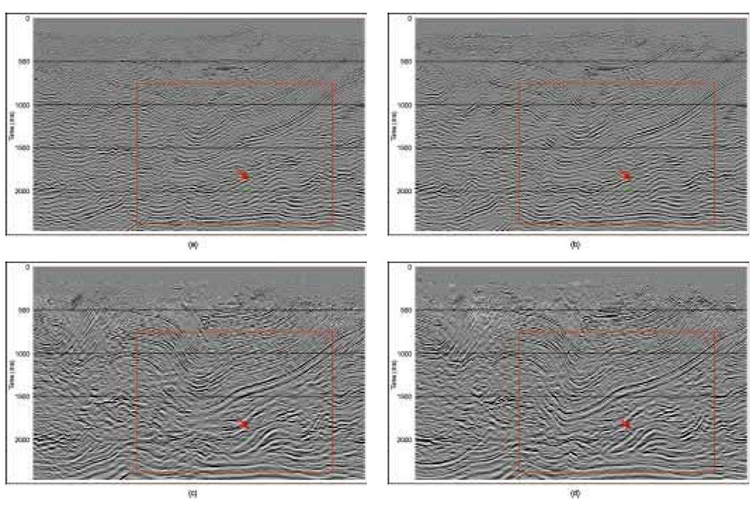
The image that we obtained from PSTM is shown in Figure 6(b). The improvement over the poststack migration is typical – better focussing throughout, with a significant reduction of structural uncertainty. For example, the shallow reflectors on the left side form a second syncline against which the major syncline terminates. Also, the objective thrust sheets are much clearer. The leftmost imbricate (the specific target for this investigation), though, is a perfect example of the old interpreter’s saying, “If I hadn’t believed it, I never would have seen it!”

For PSDM, both isotropic and anisotropic, we applied a nearsurface velocity model obtained from turning-wave tomography (with offsets up to 3600 m.) to the top of the velocity model, and we used interactive tomography to estimate velocities from deeper reflectors, as illustrated in Figure 5.

We show in Figure 6(c) our final isotropic PSDM image, displayed in time to compare with the time migrations. The PSTM image shows generally better signal quality than the isotropic PSDM image, especially at depths where the higher velocities have stretched the wavelet produced by PSDM. There are also areas where the PSTM shows a clearer structural picture than the isotropic PSDM, for example at the base of the major syncline and below it. (But there are more subtle, anisotropic reasons for this, as we shall see.) On the other hand, the PSDM shows better steep-dip imaging and more accurate imaging on the tight folds on the right side beneath the syncline. Our target prospect is much more clearly imaged on the PSDM, which finally shows a clear picture of the imbricate, indicated by the coloured arrow in Figure 6. Also, we have greater confidence in its lateral positioning. As we shall see, however, we should not be too confident yet about the lateral positioning of the target.

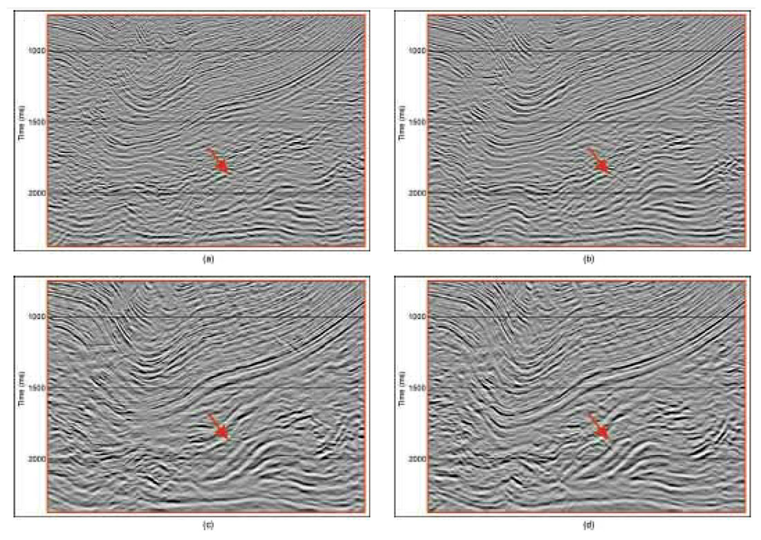
Finally, we introduce anisotropy into our model. Normally, we would introduce anisotropy in all the PSDM iterations, but here we wanted to highlight the difference between our best (at least, at the target) isotropic image and our final anisotropic image. Figure 6(d) shows the image obtained from the anisotropic PSDM. Incorporating anisotropy has resulted in significant structural improvement, tightening and focusing the syncline and producing greater continuity beneath it. It has also improved the clarity of the target thrust, and it has moved it about 150 m, giving us our greatest confidence in its position. Figures 7(a-d) show a close up sequence illustrating the progressive improvements in the imaging of the exploration target from post stack time through anisotropic prestack depth imaging.

Discussion

We have described several advanced seismic depth imaging and velocity estimation techniques that allow us to produce accurate depth images and plausible velocity models efficiently. A processing flow using these techniques is fairly natural; the steps can all be understood by a competent geophysicist, and they combine to provide an interpretive path through the maze of seismic processing.

At Blackstone, these techniques have allowed us to see details of exploration targets that eluded detection even with highquality PSTM. The exploration target is the additional imbricate that the time migrations failed to image. While the isotropic PSDM revealed the target imbricate, the anisotropic PSDM highlights it much more clearly. Applying the advanced tools gave us far greater confidence in the location of the targets, and even their very presence, than was possible with the standard tools.

None of the images is perfect, though. The poststack migration failed to image the target thrust, and the PSTM barely imaged it. All the images show a confused picture on the left side, and all show unlikely basement structure. Most likely, reflections from out of the plane contaminate the images to some degree. It might be possible to fiddle with velocities, reducing the amount of out-of-plane contamination and sharpening the image. This is fairly easy to do with PSTM, and much harder (and not necessarily desirable) with PSDM. An area receiving particular interest lately in 3D exploration is azimuthal variations of velocity which are relevant to ray tracing for turning ray tomography, analysis by manual tomography and anisotropic PSDM imaging. Still, with a certain amount of work, all the images can be improved.

Is such improvement generally worth the extra effort? In the Blackstone case, yes. In some Foothills areas, squeezing everything possible out of a migrated image is necessary to complete a geologic picture. In other areas, however, the general picture is fairly well understood, and our goal would be to fill in the details. Our standard processing flow proved inadequate for the task, but our advanced flow performed admirably, providing a high-quality final image as well as a plausible geologic model, including anisotropy.

Significantly, it took advanced tools to produce these results. The Blackstone area, though complex geologically, is characterized by good seismic data quality. Other Foothills areas are equally complex, with the added disadvantages of poor seismic data and/or poorly understood geology. In these areas, even today’s advanced imaging tools make structural interpretation an adventure, and it will take a significant advance in our tools before we can say that we’ve overcome all the imaging problems associated with Foothills geology.

Acknowledgments

The authors would like to thank Talisman Energy for permission to show the results. We also thank Ken Evans at Veritas GeoServices for performing the time processing on the Blackstone data set and Placer Deguzman for assistance with the document and images.

Acknowledgements

The authors would like to thank Talisman Energy for permission to show the results. We also thank Ken Evans at Veritas GeoServices for performing the time processing on the Blackstone data set and Placer Deguzman for assistance with the document and images.