Towards wave-equation imaging and velocity estimation

Introduction

Prestack depth migration (PSDM) has gained widespread acceptance as a tool of choice for seismic imaging in geologically complex areas. Its ability to honor lateral velocity variations gives geophysicists greater confidence in the precise location of their drilling targets on their image than they can possibly have using prestack time migration (PSTM). Associated with the seismic image is a certain amount of (sometimes hard-won) knowledge of the velocity field. A crisper image usually comes along with this knowledge. In general, the more geologically reasonable the velocities, the greater will be the confidence in the depth image.

The acceptance of PSDM is not universal, though, nor should it be. PSTM sometimes produces better images than PSDM in complex areas where velocity knowledge is scanty, and PSTM usually produces respectable images with less interpretive work than PSDM requires. Where PSDM uses its sensitivity to velocity errors as a lever to combine the seismic image with the velocity model, PSTM uses its insensitivity to produce an acceptable (but imprecise) image without a detailed estimate of velocity. So the goals of PSDM and PSTM complement each other, and the two technologies are often used in tandem in order to optimize the process of producing (1) the seismic image and (2) either the associated velocity or its uncertainty.

Although discussing the relative benefits of PSDM and PSTM is interesting, that is not the goal of this article. Rather, we focus on PSDM and its associated velocity analysis. In particular, we discuss some of the latest “cutting edge” techniques, and we argue that these are very close to being widely available. An earlier article on “bleeding edge” techniques by one of us described some cutting-edge techniques, as well as some issues impeding their use. These techniques are now beginning to provide alternatives to the standard PSDM flow of Kirchhoff migration and traveltime tomography. The new imaging techniques, Gaussian beam migration and migration by wavefield extrapolation or “wave-equation migration” (WEM), promise greater accuracy and less noise in the presence of rapid velocity variations than Kirchhoff migration. The new velocity estimation techniques, involving complete wavefields and not rays, are more consistent with WEM than ray-based tomography is. The combined use of improved imaging and wave-equation velocity analysis therefore promises a more complete and consistent approach to depth imaging, and will hopefully prove its value in the near future.

Has a single tool allowed these technologies to emerge? An obvious candidate for such a tool is the dramatic increase in computer speed over the last few years, but that is only part of the answer. Not only is WEM more compute-intensive than Kirchhoff migration, it also makes requirements on the input data that Kirchhoff doesn’t obviously make. The data sampling requirements appear to be far more stringent for WEM than for Kirchhoff, which is considered to be almost infinitely flexible. Although the apparent lack of data sampling requirements for Kirchhoff migration is a fiction, the requirements for WEM are very real. However, modern data interpolation techniques are beginning to produce data sets, fully consistent with the actual data acquired in the field, that are well-enough sampled for any migration technique. A final tool that will be very useful in imaging Foothills data, or any data where anisotropy is significant, is the emerging ability to incorporate fairly general anisotropy in Gaussian beam migration and WEM.

The need for depth imaging

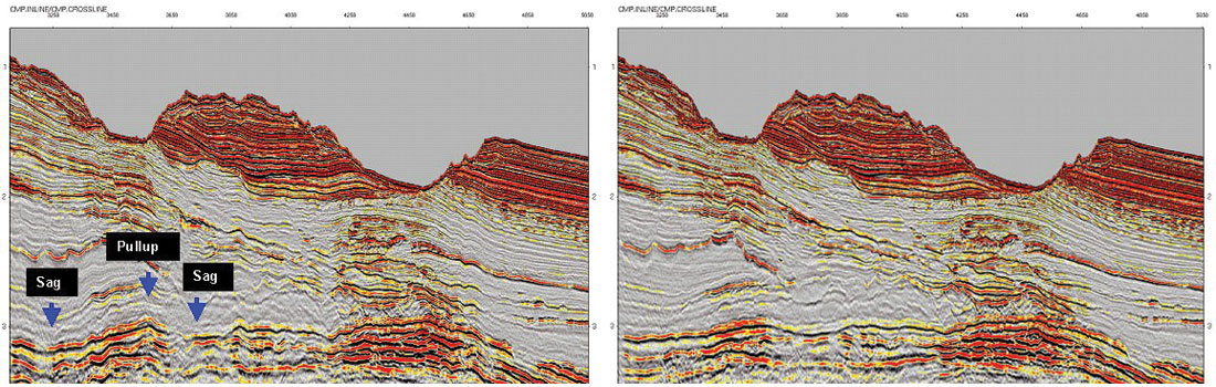
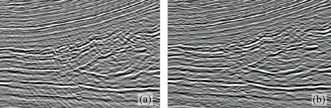
While time migration can often produce well-focused images with less work than depth migration, the accuracy of depth migration in areas of strong lateral velocity variation is always greater than that of time migration. Figure 1 compares PSTM and PSDM images from offshore East Coast Canada. Both images in Figure 1 are well-focused, but the PSTM image shows false structures – time high and lows – below the water bottom. These are due to the rapid lateral velocity variation across the water bottom canyons.

In structured areas on land, e.g., in the Foothills, the case for depth migration becomes more complicated. On the one hand, poor data quality doesn’t always guarantee that depth migration will produce a satisfactory image. On the other hand, the expense of drilling Foothills targets raises the stakes for accurate imaging. Here, the improvement in lateral positioning provided by depth migration is crucial (if the target is visible at all). Also, the additional improvement gained by incorporating anisotropy into the velocity model can spell the difference between a well that hits the target structure and one that misses, necessitating a sidetrack.

The importance of anisotropic depth migration in the Foothills became particularly evident for the problem of imaging structural targets beneath dipping shales (which occur in almost every Foothills exploration play). Shales display significant anisotropy, and the use of isotropic depth migration causes significant lateral mispositioning in the images beneath shales. Until the late 1990’s, an all-too-common effect of applying isotropic migration to data from an anisotropic Earth was a well placement in front of the leading edge of the actual target. In fact, some companies made an ad hoc allowance for anisotropy when placing wells on isotropic images, by placing their wells some hundreds of meters behind the target as mapped from the depth image. That practice seems to have died out, due to our better understanding of the effects of anisotropy. In short, accurate depth imaging requires the combination of anisotropic depth migration with an accurate anisotropic velocity model.

Depth migration of complex structures is both iterative and interpretive, with the depth reflection image and the interval velocity estimation being closely coupled processes. One requirement of a velocity model for thrust belt areas is that we be able to restore the model to its undeformed state. This process of “reverse-time geology” is called “structural balancing”; in it, we seek to produce a model whose formation volumes in the present deformed state are the same as layered formations in an undeformed layered state prior to thrust faulting. This process of structural balancing requires seismic depth models, and hence is possible with depth migrated data. (In 3-D, of course!)

Away from the Foothills, the widespread presence of shales provides motivation for anisotropic migration of Plains data. Should this be done in time or in depth? Historically, Plains data have been migrated in time, often after stack. More recently, though, several examples have shown that anisotropic PSDM produces well-focused, highly resolved images of subtle structural and stratigraphic targets. While the extra work of applying PSDM to Plains data might be hard to justify economically in some cases, the recent PSDM successes might point the way to an efficient, optimal flow for either PSDM or curved-ray PSTM for such targets. One possible way to do this is by integrating well data into the velocity model better than we’re presently doing, perhaps as part of a global tomographic velocity estimation.

Beyond Kirchhoff depth imaging: The promise and the requirements of wavefield extrapolation and beam methods

For several years, WEM has been in production use on large-scale marine projects. While Kirchhoff PSDM produces images that are more accurate, and often better focused, than PSTM images, the Kirchhoff migration operator still tends to produce a great deal of unwanted noise in areas of extreme complexity. Quite often, especially in areas of extreme complexity, WEM produces cleaner, more interpretable images than Kirchhoff migration. Figure 2 shows an example of this on a subsalt play in the Gulf of Mexico.

While WEM is more accurate than Kirchhoff migrations, it is also more computationally intensive. To reduce computational cost, production wave-equation migrations solve a one-way wave equation instead of the more general, but substantially more expensive, two-way wave equation. The computational advantages of the one-wave equation come at the price of limiting the geological dips that can be accurately imaged. The steeper the propagation angle of the reflections, the more challenging the computational task of accurately extrapolating them in depth is. In the limit, overturned reflections cannot be imaged by downward- continuation migration. Since the invention of wave-equation migration by Claerbout in the early 70’s, innumerable numerical methods for improving the angular range of downward-continuation migration have been introduced. Recently, the research focus has shifted from improving the numerical schemes to adaptating the propagation coordinate system to the true propagation direction of the events. Dip limitations can be overcome by solving the one-way wave equation along a modified coordinate system, such as a rotated Cartesian coordinate system (Shan and Biondi, 2005) or a coordinate system computed by ray tracing (Sava and Fomel, 2005).

Another practical advantage of the one-way wave equation is that the generalization of one-way wave equation migration to anisotropic media (at least with a vertical axis of symmetry) is fairly straightforward. By contrast, anisotropic two-way propagation can be completely achieved only by solving the elastic wave-equation instead of the acoustic wave equation, and consequently increasing the computational cost by at least an order of magnitude. This limitation might be soon be removed by the development of an anisotropic acoustic two wave equation along the lines described by Du et al. (2005).

Figure 3 compares the result of isotropic prestack WEM (top panel) and anisotropic prestack WEM (bottom panel). The dipping reflections are better focused by anisotropic migration than by isotropic migration. Furthermore, the Angle Domain Common Image Gathers (ADCIGs) are fairly flat after anisotropic migration, but they display a substantial residual moveout after isotropic migration. ADCIGs are the main tool for updating migration velocity after wave-equation migration. When the migration velocity is accurate, reflections are flat along the angle axis. In contrast, when the migration velocity is inaccurate, the events are either smiling upward or frowning downward. These deviations from flatness can be measured and inverted into velocity updates either by simple vertical updating or by a reflection tomography inversion. This process is commonly called Migration Velocity Analysis (MVA).

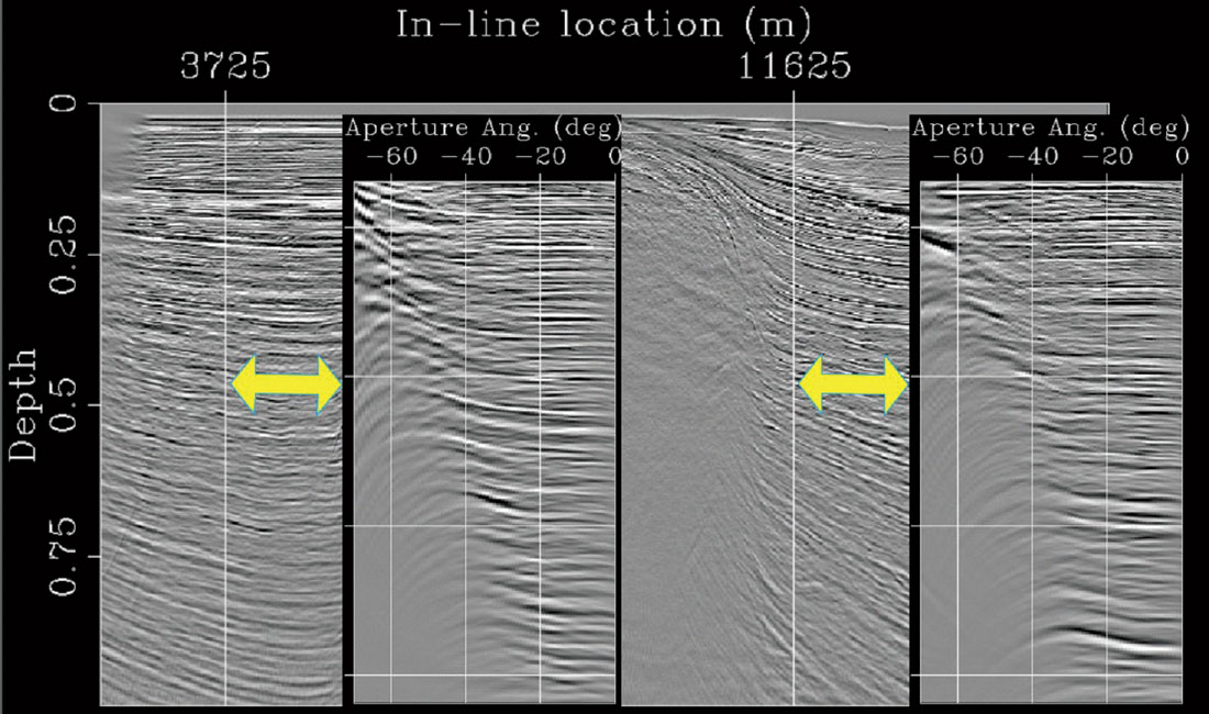
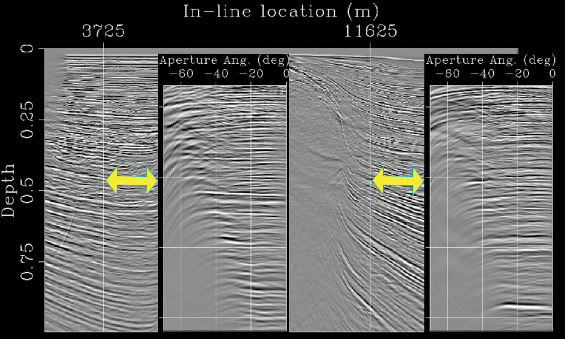
The computation of ADCIGs from isotropic wave-equation migration and their use for velocity updating has been common practice for several years. As Figure 3 illustrates, this practice can be extended to anisotropic migration. However, estimating an anisotropic velocity function is a challenging problem because of the additional degrees of freedom needed to parameterize an anisotropic model. Depending on the type of anisotropy in the rocks, we may need to parametrize the velocity function with three or four (sometimes even more) parameters at each spatial location. These additional degrees of freedom make the estimation problem even more poorly constrained than in conventional isotropic MVA.

Given the success of WEM on enormous marine projects, why hasn’t WEM taken off in the Foothills? The short answer to this question is “data sampling issues”. WEM requires a well-sampled wavefield to migrate, and Foothills acquisitions – Plains acquisitions, too – almost never sample a wavefield well enough to apply WEM. An exception is in 2-D, where tight group spacings often allow the downward continuation of shot records. In fact, Gaussian beam migration and WEM are becoming practical tools, although these techniques still need to contend with problems of crooked lines, skipped shots, and extreme surface topography that Kirchhoff migration has learned to overcome. Figure 4 compares a Gaussian beam image with a Kirchhoff image on a Foothills 2-D line, showing a reduction of noise swings in the Gaussian beam image.

In 3-D orthogonal shooting, the widely spaced receiver lines record a highly aliased wavefield at almost all seismic frequencies. We usually don’t consider this to be a problem when we apply Kirchhoff migration to 3-D land data. Strictly speaking, though, Kirchhoff migration is a wave-equation migration technique, and it is subject to the same rules that hold for other methods. Why, then, does Kirchhoff migration “work” when other methods fail? Actually, Kirchhoff migration doesn’t really work all that well either. In the receiver-line direction, where the data are well-sampled, Kirchhoff migration works well; in the orthogonal direction, it doesn’t work well. Although we apply very effective anti-aliasing techniques to the migration operator, it doesn’t have enough information to resolve the migration swings in the crossline direction into coherent geological structure at very shallow depths. With similar anti-aliasing techniques applied, we could produce equally unsatisfactory crossline shallow images using any WEM technique, but the expense of including a huge number of zero traces in the migration makes this process uneconomical.

In order to apply WEM or Gaussian beam migration of 3-D land common-shot records, we must reduce the receiver line spacing, either in acquisition or in processing. With no serious movement afoot to increase the channel count dramatically, it appears that we will need to reduce the receiver line spacing by processing, in the form of data interpolation. Fortunately, data interpolation techniques have recently evolved to the point where they can interpolate poorly-sampled, irregular data from a variety of offsets, azimuths, surface velocities, and surface elevations with some fidelity (Trad et al. 2005). We emphasize that the purpose of data interpolation is not to act as a substitute for actual acquisition, and we certainly don’t recommend drilling wells on purely interpolated data. Instead, we view interpolation as a preconditioning operation for seismic imaging process such as stack or migration: it should produce unaliased traces that are consistent with the actual acquired data. A principle of parsimony should be applied in the interpolation to guard against producing data that adds structure not present on the uninterpolated image. The interpolated traces should combine with the actual acquired traces to give the migration a chance to proceed in an unaliased fashion.

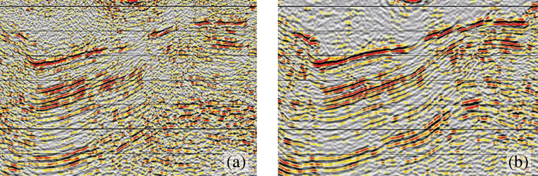
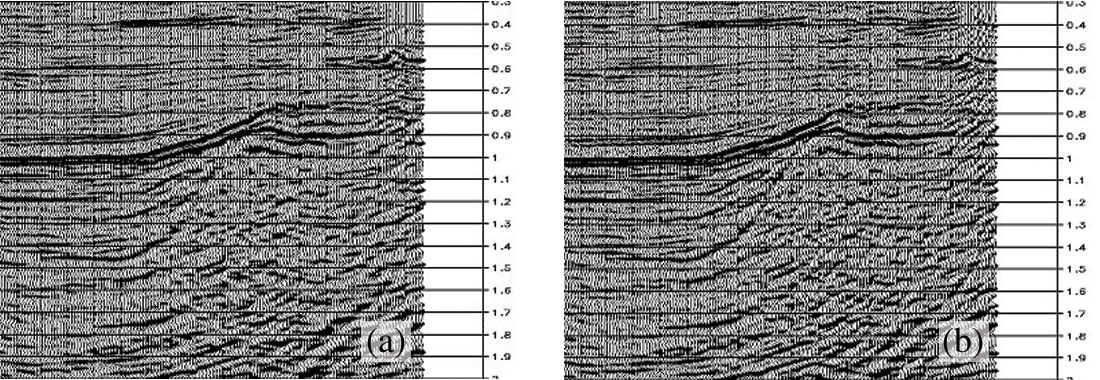
We show an example of the benefits of data interpolation in Figure 5. Although the thrust of our article is on depth migration, the images in Figure 5 are from PSTM. This land data set, acquired over a structured area in Thailand, was acquired using orthogonal shot and receiver lines. In Figure 5(a), a PSTM migration/stack was produced, and then the stack was interpolated; in (b) the data were interpolated before migration. In both cases, the objective was to improve the steep dips in the image. However, the prestack interpolation produced a data set for migration input that was better sampled than the uninterpolated data set, and this allowed the migration to operate with greater fidelity (in this case, less anti-aliasing) on the steep-dip events. As desired, the prestack interpolation did not add information to the 3-D data set, but it did allow the migration to make better value of the information that was already there.

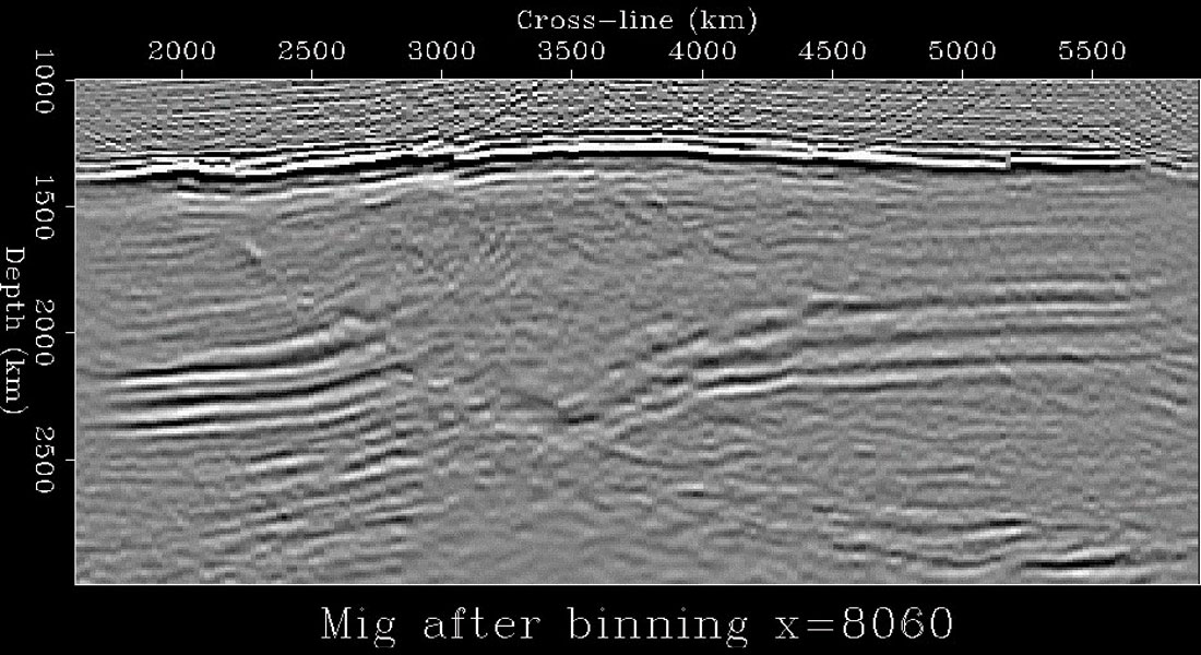
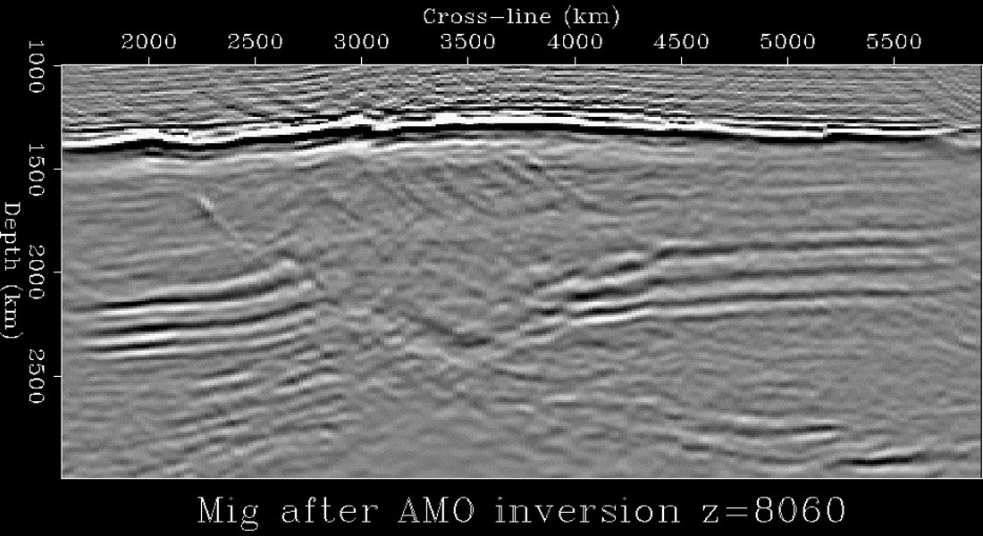
Least-squares wave-equation migration (Kuehl and Sacchi, 2002; Prucha and Biondi, 2002) is an alternative approach to data interpolation for attenuating the image artifacts caused by irregular and insufficient data sampling. The inversion of a full wavefield imaging operator is expensive and not likely to be routinely adopted unless the imaging artifacts caused by irregular acquisition geometry are compounded by illumination problems related to complex overburden, such as in the subsalt or possibly below complex over-thrusts. However, least-squares inversion of the time-imaging operator or partial-migration operators can be effective in overcoming poor spatial sampling, and they are becoming computationally affordable (although still expensive compared with data interpolation). Well-sampled zero- offset cubes can be obtained by inverting the DMO operator (Ronen, 1987), and well-sampled prestack data can be obtained by least-squares inversion of the AMO operator (Chemingui and Biondi, 2002). Figure 6 shows the advantages of inverting the AMO operator in the frequency-wavenumber domain before wave-equation migration of a marine data set severely affected by cable feathering during acquisition. The top panel shows a cross-line section obtained using simple binning to regularize the data before migration. The bottom panel shows the same section when the data were regularized by least-squares AMO before migration. The chalk layer is heavily faulted between the depth of 1.5 and 2 kilometers. The fault blocks are easily interpretable in the image obtained after least-squares regularization, whereas artifacts hamper the interpretation in the top image.

The most “cutting edge” imaging method, although it is also one of the oldest, is reverse-time migration. Reverse-time migration is as general as the wave equation we wish to use in our algorithm. The wave equations can be 3-D, anisotropic, elastic and applied in prestack mode. The wave equation has the interesting characteristic that time can run forward or backward to produce a solution. In reverse-time, we can consider that the wavefield can be depropagated back to reflectors. The wave equation is approximated by a finite- difference formulation, and accuracy requires a fine spatial grid and time sampling small enough to avoid instability. Coding is generally straightforward, even with higher- order solvers. Finite- difference solutions will include reflections, refractions, diffractions, multipathing and basically all wave phenomena described by whatever version of the wave equation we may choose to use. The method has been successfully used to image salt flanks and overturned beds in thrust fault environments. With a good velocity model, it can produce excellent results.

However, the generality of reverse-time migration comes with a cost. First, it is typically the most expensive of migration methods. Unless the velocity is smoothed, or impedance contrast set to zero by manipulation of density, it may produce unwanted interbed multiples during the depropagation of the wavefields. In order to accommodate low velocities (shorter wavelengths), it often requires a fine computational grid in order to avoid grid dispersion. Unlike Kirchhoff migration, we cannot easily break the subsurface into small chunks; the solution must be achieved globally. The large computing times can be somewhat obviated by the use of parallel computing. However, unlike Kirchhoff migration, parallelizing finite-difference solvers is not trivial since different blocks of velocity cells must communicate with each other in the wave equation computations. Finally, as mentioned above, accommodating anisotropy (an elastic effect) is difficult using an acoustic two-way wave equation. However, some progress has been made on this front. In summary, reverse-time migration is general and straightforward to code but is expensive and computationally demanding; also, it can produce artifacts that are hard to control. We expect these issues to be overcome to some degree in the next few years.

Depth migration velocity estimation, using rays and waves

When the overburden is complex and geometrical rays poorly approximate finite-frequency wave-propagation, we image the data with wave-equation migration. In these cases we would also like to use a wave-equation operator to estimate velocity, because ray-based reflection tomography might yield inaccurate and unreliable results. Progress has been recently achieved towards the development of wave-equation MVA methods, though none of the presently available methods is ready for production processing on 3-D data. Pratt and his students (Sirgue and Pratt, 2004) have shown that a frequency-domain implementation of “classical” waveform inversion (Tarantola, 1986) can be effective in estimating the velocity model when refracted arrivals are recorded at long offsets. Wave-equation operators can be also used in methods closer to conventional MVA than waveform inversion. Methods such as Differential Semblance Optimization and Wave-Equation MVA (WEMVA) (Sava and Biondi, 2004) aim at maximizing the focusing of the image by minimizing departure from flatness of the events in ADCIGs. We expect these promising research directions to lead to effective practical methods in the near future.

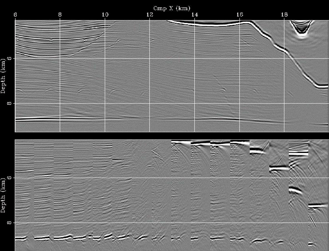
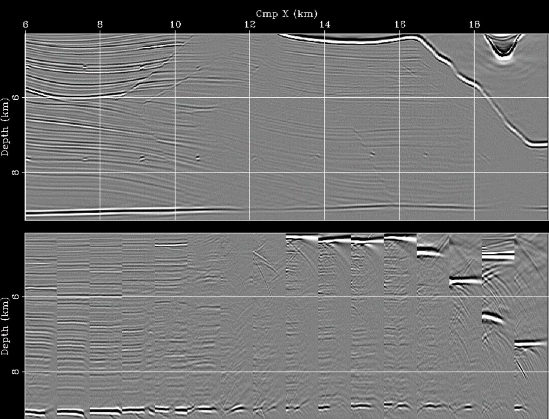
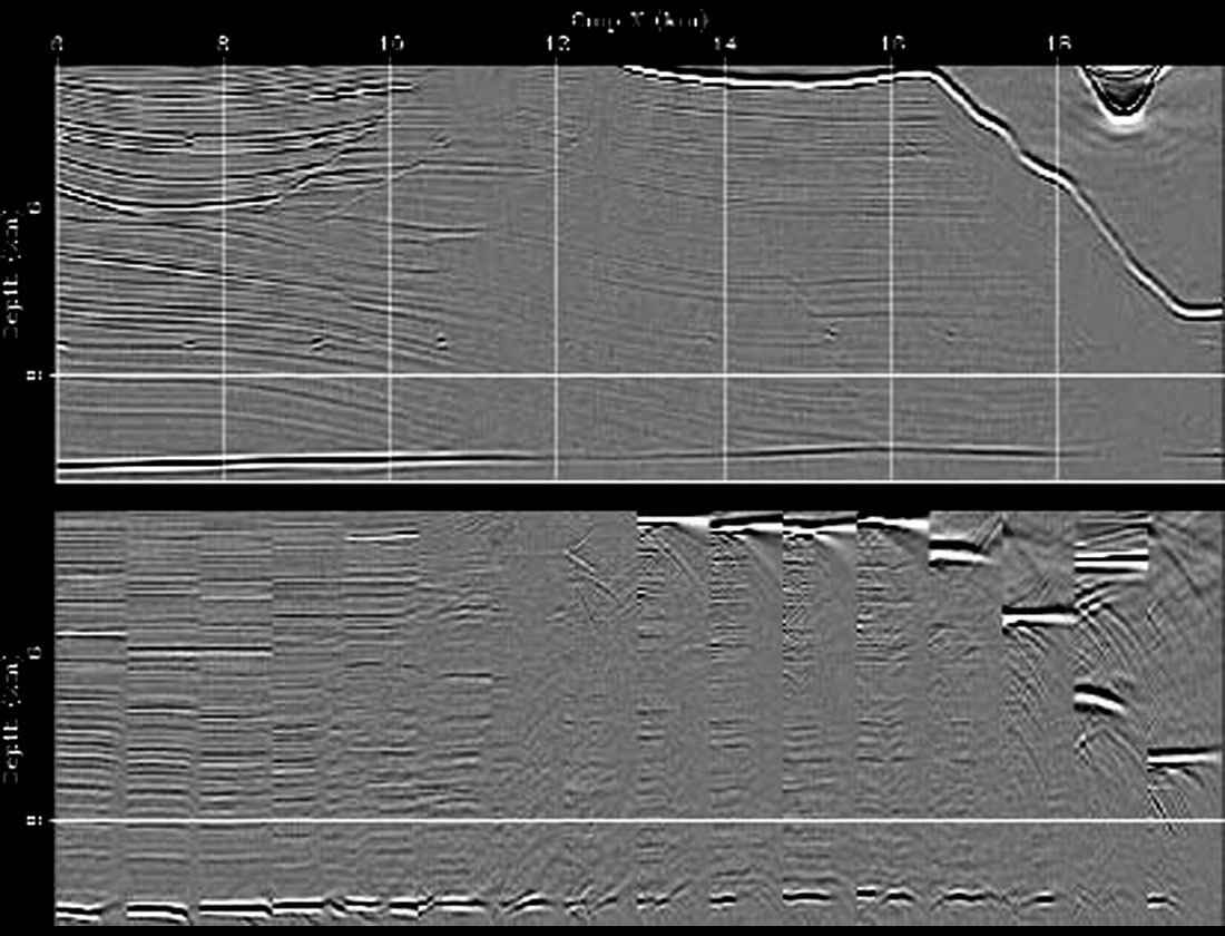
Figure 7 shows the results of applying WEMVA to the estimation of velocity in the subsalt area of a complex synthetic model (the Sigsbee model distributed by the SMAART JV). The figure shows the migrated images and the corresponding ADCIGs taken at regular spatial intervals. The top panel shows the image obtained by wrongly assuming a low-velocity anomaly in the subsalt. The image is poorly focused and the ADCIGs smile upward. After WEMVA the image is well focused and the ADCIGs are fairly flat (middle panel). The position of the reflectors and the flatness of the ADCIGs are similar to the results obtained using the correct velocity model shown in the bottom panel. Notice that below the steeply dipping salt flanks the subsurface is poorly illuminated and the ADCIGs are discontinuous and not perfectly flat even when the migration velocity is the one used for modeling. These errors are due to incomplete illumination of the subsalt reflectors by the surface seismic sources and receivers. The interplay between incomplete reflector illumination and velocity estimation is likely to represent a challenge for our imaging algorithms even in the future.

Conclusions

The use of PSDM is routine in many parts of the world (e.g., in the Gulf of Mexico and the Canadian Foothills), and is becoming more widespread. WEM and Gaussian beam migration have demonstrated more accurate and less noisy images than Kirchhoff PSDM can provide, and their use is also becoming more widespread. In some areas, however, PSDM has historically been limited to the application of Kirchhoff migration. For example, Foothills areas, with their sparse data acquisition and anisotropic shales, have been considered to be suitable only for Kirchhoff PSDM. Recent advances in data interpolation have enabled us to consider applying WEM and Gaussian beam migration to Foothills data as well as other data with acquisition challenges. Also, recent advances in anisotropic WEM give us a choice of advanced imaging methods to use in areas with dipping shales. Still a few years from production use is full-blown least-squares migration, which might overcome (1) deficiencies in acquisition (as does data interpolation today) and (2) deficiencies in subsurface illumination (which no present imaging method completely accomplishes at present).

As an adjunct to more accurate depth imaging, velocity estimation techniques that are based on waves, not rays, are emerging. These come in a variety of flavors, including waveform inversion of long-offset data and wave-equation MVA applied to ADCIG’s. Although these tools are not yet ready for production use as full-wave processes, some of them have versions that can presently be used with rays. One such method is tomography using subsurface dip and opening angles measured from the stack and ADCIG’s.

For more than two decades, progress in depth imaging has been incremental. The accumulation of these incremental advances has enabled geophysicists to use seismic data to see drilling targets beneath complex overburden. Since the earlier (2003) “bleeding edge” article, advances such as data interpolation and anisotropic WEM have been realized, and should soon help geophysicists to see targets that are invisible today

Acknowledgements

We thank PTT for permission to show the Thailand data. We thank Veritas, specifically J. J. Wu and Jerry Young, for permission to show the East Coast Canada and Gulf of Mexico examples. We thank Bob Clapp for providing the images in Figure 6.