Study of elastic anisotropy on an unconventional ‘shale’ rock using ultrasonic waves and static strain measurements

Elastic anisotropy is a seismic attribute defined as the variation of wave speed as a function of its propagation direction within a medium. With the increase in interest of unconventional reservoirs, the incorporation of anisotropic factors is a necessity to provide more accurate seismological models. Without consideration of anisotropic effects, sub-surface imaging (especially from wide-azimuth and far-offset data) can produce erroneous anomalies and lead to misinterpretation (Wild, 2011). Although reflection seismic data can provide insight into the anisotropic velocity fields (Alkhalifah & Tsvankin, 1995), laboratory studies at the core scale are ideal for characterizing the magnitude of anisotropy as it allows for greater control and precision of the testing conditions.

These measurements are important to study the anisotropy of the rock and the relationship to its petrophysical properties where they may be observed at the seismic scale. In this study, ultrasonic velocity measurements are conducted on Duvernay shale samples to gain insight into that formation’s elastic properties.

Background

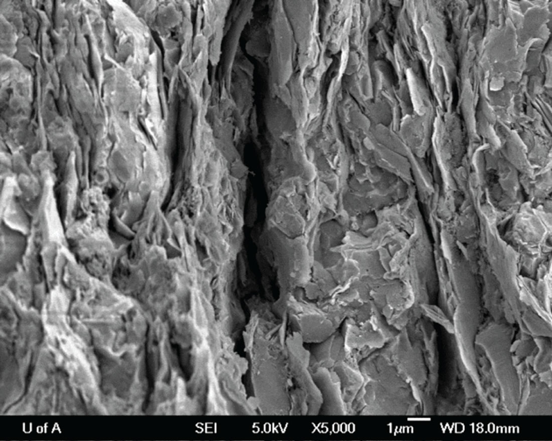
Shales tend to make up a substantial component of the average sedimentary basin by volume (Johnston & Christensen, 1995; Jones & Wang, 1981) and are presently utilized as reservoir rocks. They also tend to exhibit a relatively large degree of anisotropy as the orientation of microcracks, preferential clay platelet alignment, and layering all contribute significantly to this phenomenon. Such features can be seen in Figure 1.

We model the overall elastic compliance of the rock as

where is the compliance of an anisotropic medium void of compliance cracks and is the excess compliance due to the clay platelet contact regions (Sayers & Kachanov, 1995; Mavko, et al., 2009). In addition, Sayers (1999) showed that these cracks are more compliant in shear than in compressional stress. Therefore, at large values of hydrostatic stress where these contact regions of the clay platelets close, we assume the rock to have an elastic compliance of and inversely, an elastic stiffness . Schijns, et al. (2012), for example, have recently used this theory to show that cracks must be considered in the overall anisotropy of a thick formation from comparisons of laboratory and walk-a-way vertical seismic profile measurements.

Here, we make the assumption that the samples are homogeneously transversely isotropic with a vertical axis of symmetry (VTI). For this case, the elastic stiffness tensor is of the form (King, 1970)

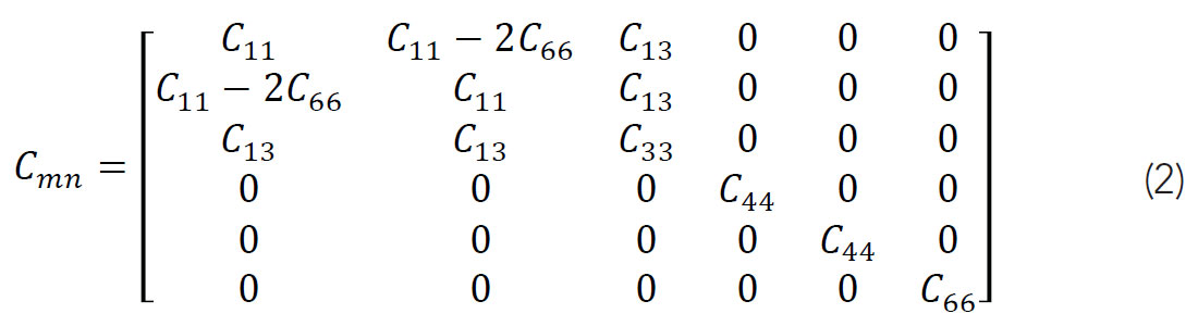
where C is the Voigt elastic stiffness matrix with 5 independent elastic constants. Equivalently, Equation 2 can be expressed as the elastic compliance tensor with elastic moduli more familiar to the engineering community (Meléndez-Martínez, 2014)

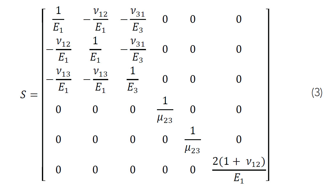
where E is the Young’s modulus, ν is Poisson’s ratio, and μ is the shear where the subscripts denote the 3 orthogonal axes X₁, X₂ (perpendicular to symmetry axis) and X₃(parallel to symmetry axis). More specifically, the Young’s modulus E₁= E₂ is the ratio of the uniaxial stress applied to the isotropy plane to its strain along the same axis. E₃ would be the same ratio, but with stress applied and strain measured perpendicular to the isotropy plane. The shear modulus μ₂₃ is defined as the ratio of shear stress to shear strain in the X₂ direction on the plane with a normal in the X₃ direction. Poisson’s ratio is defined as the negative ratio of transverse to axial strain where ν₃₁ corresponds to the stress applied perpendicular to the isotropy plane ( X₃ ) with strain measured parallel (X₁ = X₂) . Similarly, ν₁₂ corresponds to stress applied parallel to the isotropy plane with strain measured parallel as well (Sayers, 2013).

From the elastic constants, Thomsen’s parameters of anisotropy (Thomsen, 1986) can be calculated for a VTI medium

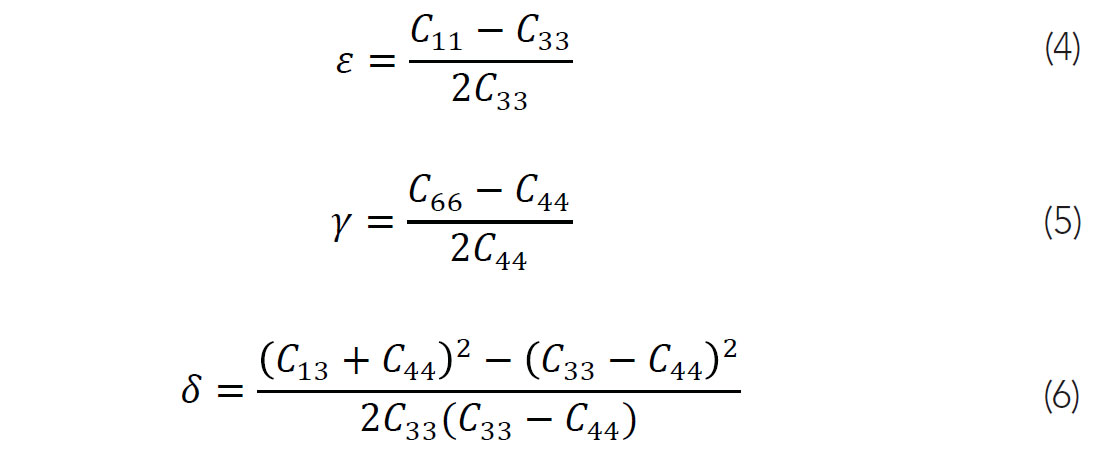
where and are dimensionless parameters used to qualify the P-wave and S-wave anisotropy respectively. The parameter can be viewed as the anellipticity of the P-wavefront.

For estimations of the elastic constants needed to fully describe transversely isotropic media, Daley & Hron (1977) derived expressions of the 3 phase velocities and as a function of the phase angle and from these expressions, we have

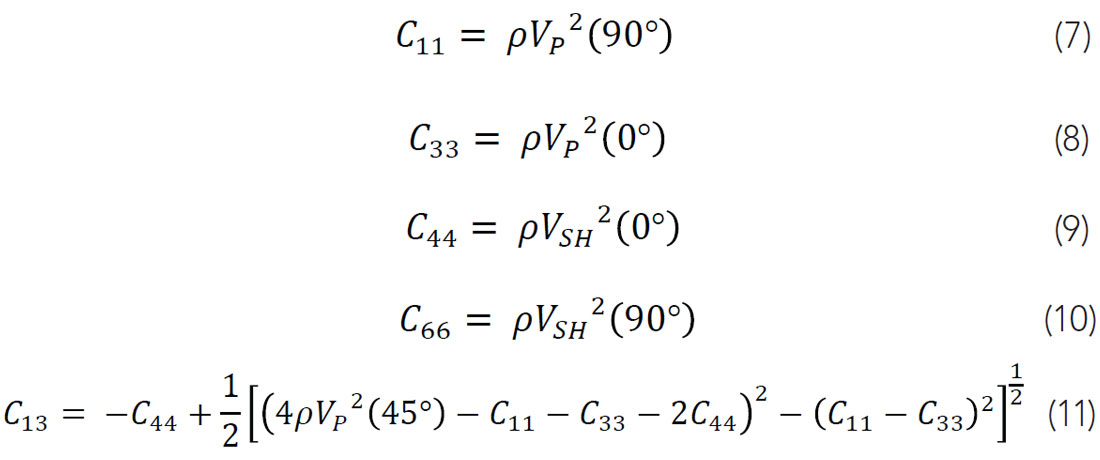
where ρ is the bulk density of the material, and the subscripts P, SH, and SV refer to the P-wave, horizontally polarized S-wave, and vertically polarized S-wave respectively. These equations allow us to estimate the elastic constants through the ultrasonic wavespeeds with the variation of the propagation direction. Examination of Equations 7-10 show that most of the elastic moduli can be determined relatively accurately by simple measurements of wave speeds along principle axes of the material. Determination of C₁₃, however, is not easily achieved in practice as propagation of errors through Equation 11 results in large uncertainties.

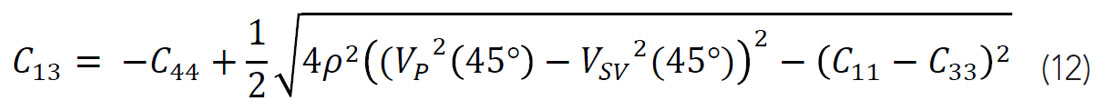
An alternative equation for C₁₃ can be derived by revisiting the phase velocity equations from Daley & Hron (1977). Hemsing (2007) proposed Equation 12 to greatly reduce the uncertainty by removing the influence of several elastic constants. The expression, instead, makes use of the 45° vertically polarized shear velocity in addition to the 45° P-wave velocity.

Methodology

In this contribution, the degree of anisotropy is investigated experimentally using the Pulse Transmission Method using piezoelectric ceramic transducers (Bakhorji, 2010; Hemsing, 2007; Kebaili, 1997). These transducers produce an impulse with the application of an electric potential, which when mounted on the surface of a sample will propagate through as an elastic wave. Upon reaching the other side, another transducer mounted to the surface converts this mechanical disturbance back to a voltage due to its piezoelectric properties. Taking the ratio transducer offset to the travel time of the signal through the sample gives us an estimation of the phase velocity at ultrasonic frequencies.

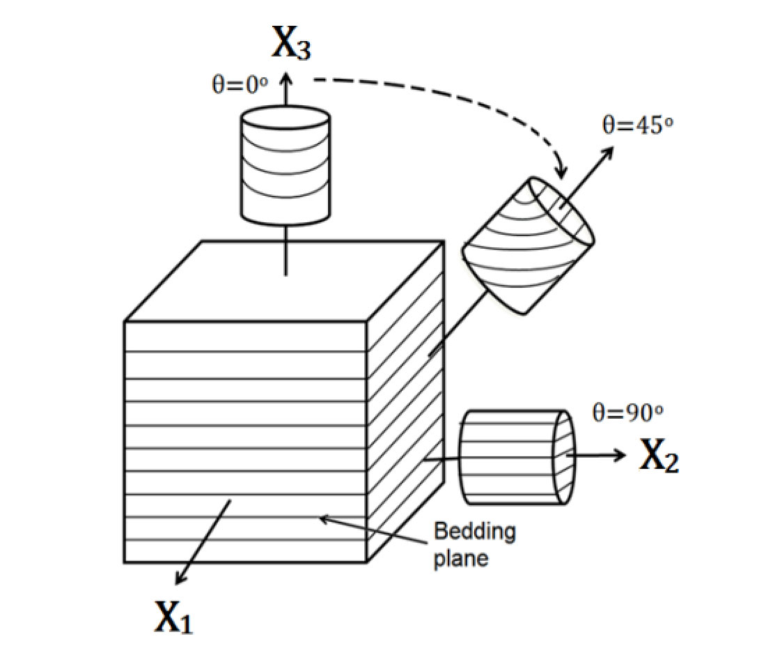
These elastic constants can be estimated from bulk density of the material and the P-wave and S-wave phase velocities measured perpendicular (V_P (0°)), parallel (V_P (90°), V_SH(90°)), and 45° parallel (V_P(45°), V_SV(45°)) to the foliation plane. The most common method of measuring these velocities is through the production of 3 cylindrical cores obtained from the main sample (Figure 2) as carried out for example by Meléndez-Martínez & Schmitt (2013). For this study, we will instead adapt a single prismatic sample configuration after Wong, et al. (2008) and Meléndez-Martínez (2014).

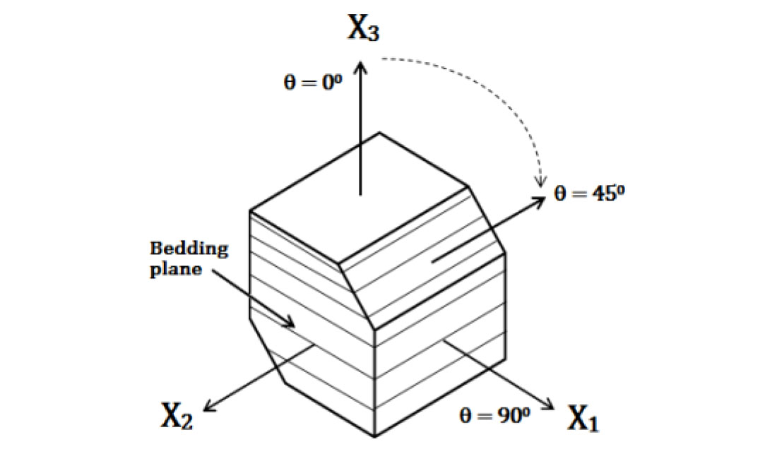
The sample configuration consists of cutting the material into a prism-like geometry (Figure 3) as opposed to the traditional 3 cylindrical cores, where each opposing face is cut to provide the propagation directions needed to estimate the elastic constants of a VTI medium (0°, 45°, and 90° to bedding). This configuration allows us to overcome the heterogeneity issues of measuring the velocities through multiple cores and reduces issues associated with attempting to core weak materials in set directions.

The setup consists of attaching copper pads directly to the sample to act as common grounds for the transducers. The transducers themselves are then glued onto the copper pads using a silver conductive epoxy with another copper pad on top acting as the positive ground. For static measurements, linear foil strain gauges are mounted parallel and perpendicular to sample bedding to measure deformation. Wires are soldered onto each electrode and dried before the application of a non-conductive urethane compound around the sample. The compound is used as a membrane to protect the transducers and sample material from the confining fluid of the pressure vessel as the samples are measured under dry and undrained conditions. Figure 4 shows a picture of the completed sample before the application of the compound. The entire sample is then placed into the pressure vessel with wires fed out through the top and connected to a data acquisition setup consisting of an oscilloscope, power supply, pulser / receiver, and digitizer.

Bulk density values of the samples were obtained from Mercury Intrusion Porosimetry.

Results

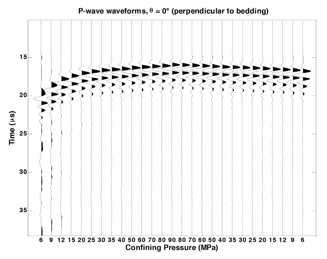
In this section, the phase velocities as well as estimations of the static and dynamic moduli of one sample are shown as results of the experiment. Figure 5 shows the P-wave waveforms for the propagation direction perpendicular to bedding. Changes in arrival time with increasing pressure can be observed directly from this figure.

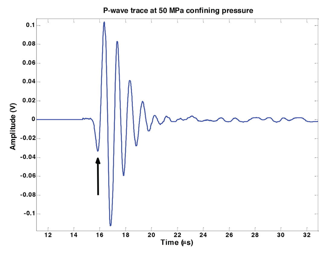
Travel times are picked from the first extremum of each waveform and are marked by arrows in Figure 6. These times are then shifted to the first break through a calibration to achieve proper timing. For additional details on this calibration, refer to Meléndez-Martínez (2014).

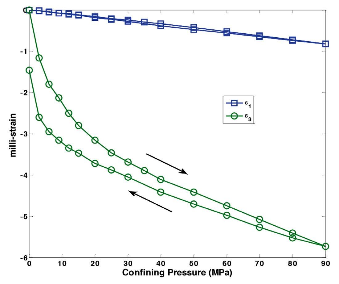
In addition to the ultrasonic velocities, deformation is measured parallel and perpendicular to the bedding plane (Figure 7). These strain values will be used to calculate the static elastic moduli for comparison with their dynamic equivalent.

Discussion

Figure 8 plots the phase velocities as a function of the confining pressure with arrows showing the progression of measurements in the pressurization and depressurization cycles.

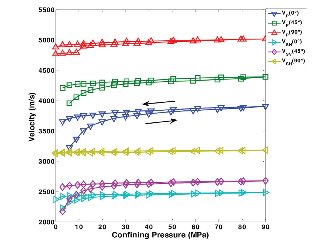
The observations in the velocities are consistent with what would be expected for a medium with vertical transverse isotropy where V_P (0°) < V_P (45°) < V_P (90°), and V_SH (0°) < V_SV (45°) < V_SH (90°). All velocities increase with confining pressure and the sample becomes stiffer due to the closure of microcracks and fractures in the rock. As a result, the anisotropy also decreases with confining pressure (Table 1), though at high pressures, the large discrepancies between the velocities show that these microcracks and fractures only account for a small source of anisotropy.

In addition to these trends, a hysteresis effect is observed in all measurements due to the microcracks and fractures closing at a faster rate during pressurization than opening during depressurization (Hemsing, 2007).

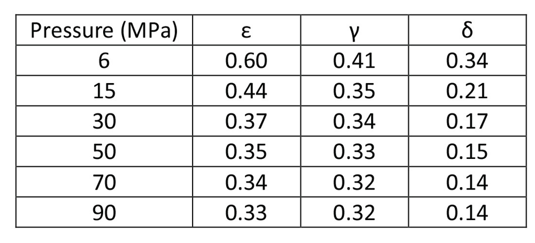
Table 1 shows the Thomsen (1986) parameters of anisotropy calculated from the estimated elastic constants where ε and γ are the P-wave and S-wave anisotropy parameters respectively.

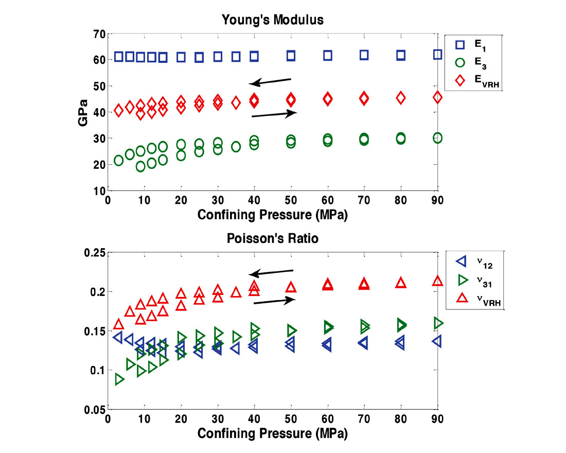
From the elastic constants, dynamic Young’s modulus and Poisson’s ratio are calculated with both single crystal and polycrystalline aggregate assumptions (Figure 9).

The numerical subscripts denote the orthogonal directions X₁, X₂, and X₃ of variables calculated with the single anisotropic crystal assumption. The subscript VRH refers to the Voigt-Reuss-Hill arithmetic average of the upper Voigt and lower Reuss bounds (Hill, 1952) to provide an estimation of the effective isotropic elastic moduli when considering a polycrystalline aggregate. These values are shown as a reference for the moduli calculated with single crystal assumptions.

As expected for shales, the discrepancy in values of Young’s modulus shows that the sample is stiffer in the X₁ direction (parallel to bedding) than in X₃ (perpendicular to bedding). However, Sayers (2013) examined the relationship between ν₃₁ and ν₁₂ and found that their ratio can be greater than, equal to, or less than 1. An inequality of ν₃₁ > ν₁₂ is expected for a partial alignment of clay particles where as ν₃₁ < ν₁₂ may indicate the presence of kerogen inclusions, microcracks, or low aspect ratio pores parallel to the bedding plane.

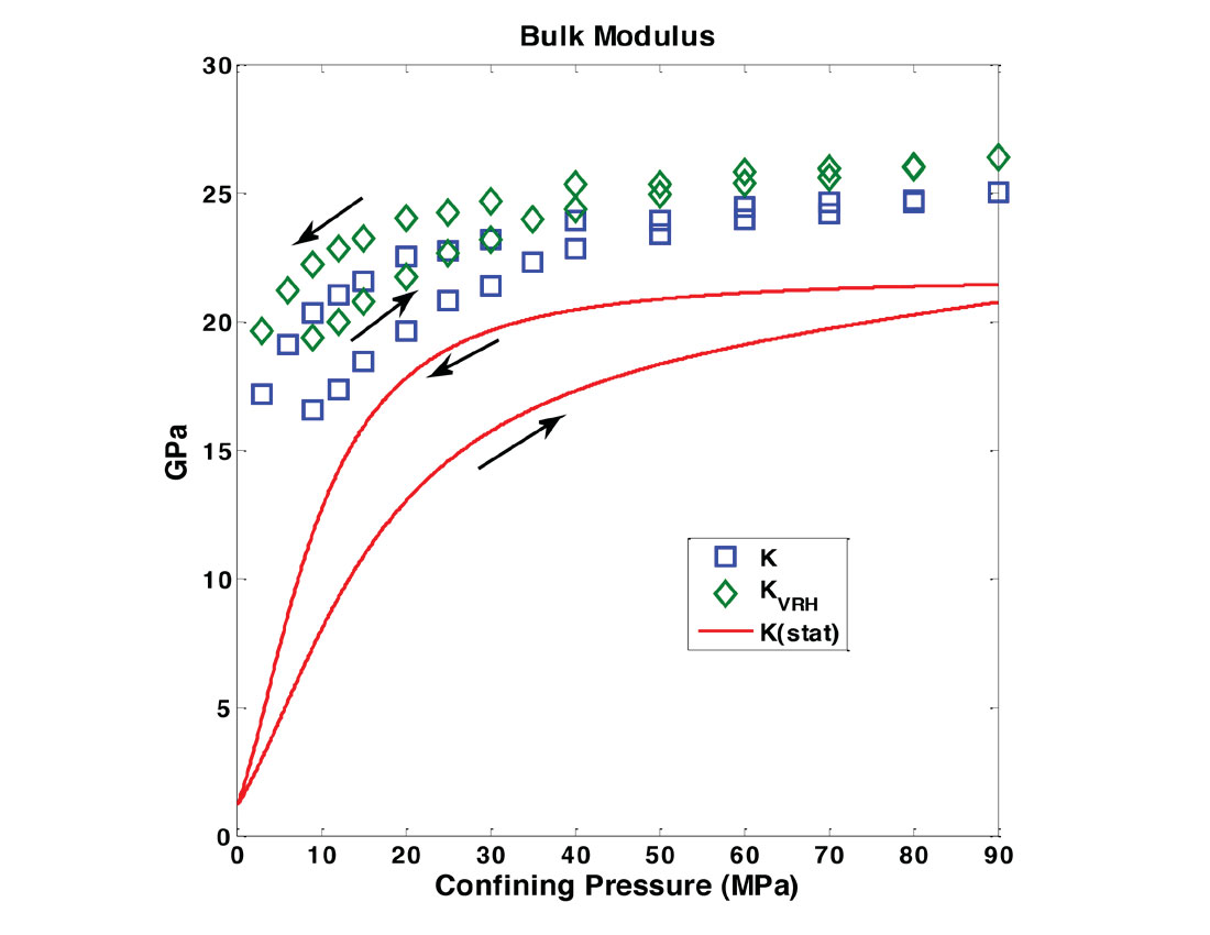
Dynamic and static tangent bulk modulus values were also calculated and plotted as a function of confining pressure in Figure 10. As expected, the static measurements are lower than the dynamic measurements where the physical causes can be attributed to the nonlinearity of the stress-strain relation where the ratio differs between measurement over large and small strains. These discrepancies can also be attributed to the sample’s inelasticity or the presence of microcracks (Mavko, et al., 2009; Cheng & Johnston, 1981).

Conclusions

Ultrasonic velocities experiments were conducted on Duvernay shale samples to investigate their elastic properties with the assumption that the material is transversely isotropic with a vertical axis of symmetry; velocities increase with confining pressure and are consistent with this assumption. Calculated Thomsen’s parameters of anisotropy showed the P-wave anisotropy ε decreased from 0.60 at low pressures to 0.33 at high pressures. Similarly, S-wave anisotropy γ decreased from 0.41 to 0.32.

Plots of the dynamic Young’s modulus and Poisson’s ratio showed that with increasing confining pressure, the closure of microcracks and low-aspect ratio pores result in the sample becoming stiffer. This effect may be indicated by the ratio ν₃₁ / ν₁₂ decreasing from greater than 1 to less than 1.

Acknowledgements

We would like the University of Alberta, Institute for Geophysical Research, and the Natural Sciences and Engineering Research Council of Canada (NSERC) for their generous support. We would also like to thank the Alberta Geological Survey for providing the samples needed for this study.