Some current workflows in shale gas reservoir characterization

Summary

With the emergence of the shale gas resources as an important energy source, the characterization of mudrocks has gained significance. To be a good resource, mudrocks need to contain sufficient organic content and respond effectively to hydraulic fracturing. Variations in total organic carbon, as well as brittleness which is a function of mineralogy, influence the compressional velocity, shear velocity, density and anisotropy of the mud rock. It should therefore be possible to detect changes in TOC and brittleness from the good quality surface seismic data. Besides TOC and brittleness, different shale formations have different properties in terms of maturation, gas-in-place, and permeability, which with proper calibration with well measurements, may be estimated statistically using surface seismic data.

Introduction

In the last decade and more, shale gas resources have emerged as not only a viable but also one of the more significant new energy sources. This viability was first demonstrated using newly perfected methods of hydraulic fracturing and horizontal drilling on the Mississippian Barnett Shale in the Fort Worth Basin. Given this initial success, geoscientists began to look for other shale basins in the US and soon the Devonian Antrim shale of the Michigan Basin, the Devonian Marcellus Shale of the Appalachian Basin, the Devonian New Albany Shale in the Illinois Basin and the Cretaceous Lewis Shale in San Juan Basin were explored and developed. Following these, the Fayetteville Shale in Arkansas, the Woodford Shale in Oklahoma, the Muskwa Shale in the Horn River Basin, and the Montney Shale, both in British Columbia, Canada, the Haynesville Shale in northwest Louisiana and east Texas, and the Eagle Ford Shale in south Texas were developed.

The development of these shales changed the traditional approach geologists had been following – that of the sequence of gas first being generated in the source rock, followed by its migration into the reservoir rock in which it is trapped. Shalegas formations are the source rock, reservoir and seal. There is no need for migration and since the permeability is near zero, it forms its own seal. The gas may be trapped as free gas in natural fractures and intergranular porosity, as gas sorbed into kerogen and clay-particle surfaces, or as gas dissolved in kerogen and bitumen (Curtis, 2002).

Such self-sourcing shale formations are commonly referred to as unconventional shale reservoirs. A more accurate word might be mudrock (Hart, 2013), since many shale source rocks do not respond well to hydraulic fracturing, either because they are too ductile, or because they quickly deform about the proppant, closing any fractures due to completion. Indeed, the minearology of most commercial shale reservoirs contains than 50% quartz and/or carbonate. The first thing that we realize in these unconventional shale reservoirs is that they have lower permeability than our conventional reservoirs. It may not be possible for the hydrocarbons to migrate within these formations, and would need stimulation in the form of hydraulic fracturing so as to release the oil and gas. Secondly, we do not need to map discrete structural and/or stratigraphic traps; these unconventional reservoirs are regionally pervasive accumulations. Although pervasive, these reservoirs are not uniform. There are optimal levels in which to land a horizontal well, TOC and brittleness varies laterally, and geohazards such as small faults need to be avoided.

To assess the prospectivity of these reservoirs, a criterion comprising the following elements could be followed:

1. Type of shale: i.e. whether it is a marine or a non-marine shale. Marine shales have low clay-content, are high in brittle minerals such as quartz, feldspar and carbonates and so respond better to hydraulic stimulation.
2. Depth: has a bearing on the generated hydrocarbon. Gas for example, is generated as biogenic gas by the action of anaerobic micro-organisms during the early burial phase, or as thermogenic breakdown of kerogen at greater depths and temperatures. Generally, a useful depth criterion for shale gas would be between 1000- 5000 m. Areas shallower than 1000 m would usually have lower pressures and gas concentrations while areas below 5000m often have reduced permeability that translates into higher drilling and development costs.
3. Thermal maturity: refers to the degree of heat and the time in the “oven” to which the formation has been exposed resulting in the breakdown of kerogen into hydrocarbons. The indicator for this measure is called vitrinite reflectance and has typical values ranging from 1% to 3%.
4. Total organic carbon (TOC): refers to the organic richness of the formation in terms of the organic material such as microorganism fossils and plant matter that provide the carbon, oxygen and hydrogen for generating the oil and gas. Typical values are equal to or greater than 1%. The TOC and thermal maturity of source rocks is assessed by means of lab analysis.
5. Permeability: refers to the fluid storage and transmissivity characteristics of a shale formation. Shale permeability is low and so artificial stimulation, e.g. hydraulic fracturing, is required to facilitate the flow of hydrocarbons into the well bore. It is important to map the intensity and orientation of natural fractures if they exist in the formation of interest. If open or poorly cemented, stimulation will “pop open” these previously generated zones of weakness. In some cases tightly cemented fractures can form fracture barriers.
6. Mineralogy: The mineral composition in shale rock formations can be wide-ranging. In a new area, one should attempt to acquire some core for an initial analysis. Electron capture spectroscopy (ECS) logs provide an initial estimate of mineralogy, but not of the form of the mineral (e.g. granular vs. cryptocrystalline) which also plays a role in brittleness behavior. One best practice is to construct a ternary diagrams of quartz, total clay and total carbonate, and map it to elastic parameters such as E (Young’s modulus) and Poisson’s ratio, resulting in a brittleness template. Such templates can then be calibrated to microseismic event location, production logs, and production itself to assess the brittleness or the ductility of the formation and how efficiently the induced fractures have stimulated it.
7. Fluid in place: is usually calculated from the pressure, temperature, porosity and the TOC for assessing the economics of the play.

An optimum combination of these elements leads to favorable productivity.

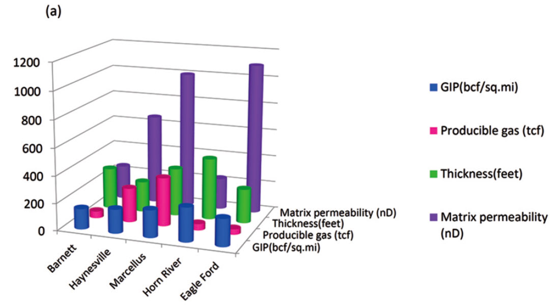
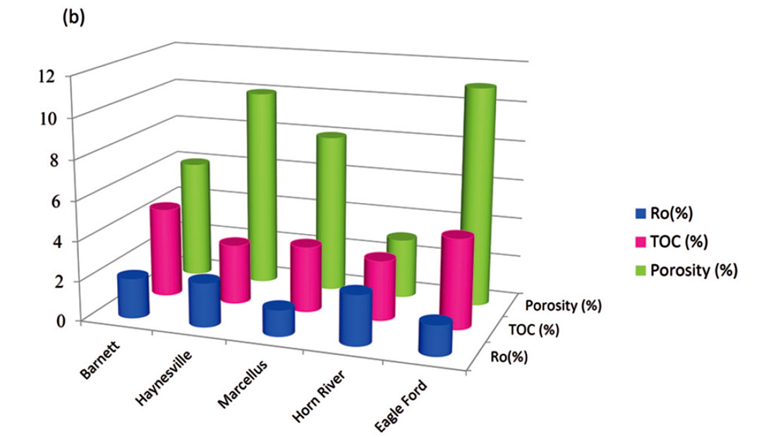
For successful exploitation of shale plays, the challenge is to determine the lateral and vertical variations in the shale reservoir, as well as determine the reservoir matrix properties such as porosity, mineral composition, TOC content and brittleness. In Figure 1 we show a comparison of some of these factors for five different shale gas reservoirs. Notice the differences in each of them. Brittle shales respond better to hydraulic stimulation, often exhibit natural fracture swarms, and so are likely to be more productive. Besides the fact that shales are heterogeneous in nature, the in situ stresses acting on the shale reservoirs and their variation need to be determined. In brittle rocks, under isotropic stress conditions, fractures propagate in a random manner. Typically the maximum stress is associated with sediment loading as it is near vertical. The addition of residual or present day tectonic stresses results in fractures that align perpendicular to the minimum (easy to open) stress direction, and hence parallel to the maximum horizontal and vertical stress directions. Such properties can often be determined from induced fractures on image logs, dipole sonic logs, and oriented core. Away from the wells, different geophysical workflows need to be applied on 3D surface seismic data. We discuss some of these workflows below.

Three-dimensional seismic data are being increasingly used in the form of different kinds of attributes providing information on fault/fracture characterization, geomechanical properties that include reservoir sweet spots, rock mechanical properties and stimulation optimization and localized stress estimates. Needless to mention, all these derived seismic attributes need to be calibrated to the available borehole and production data.

Fault/fracture characterization

Natural fractures in shale formations can provide permeability pathways and so need to be characterized, if they exist. While many shale formations may be devoid of such natural fractures, others such as the Woodford Shale have undergone significant deformation resulting in tightly spaced faults and joints. The Eagle Ford Shale as well as the Muskwa-Otter-Park–Evie Shale package in the Horn River Basin also exhibit natural fractures.

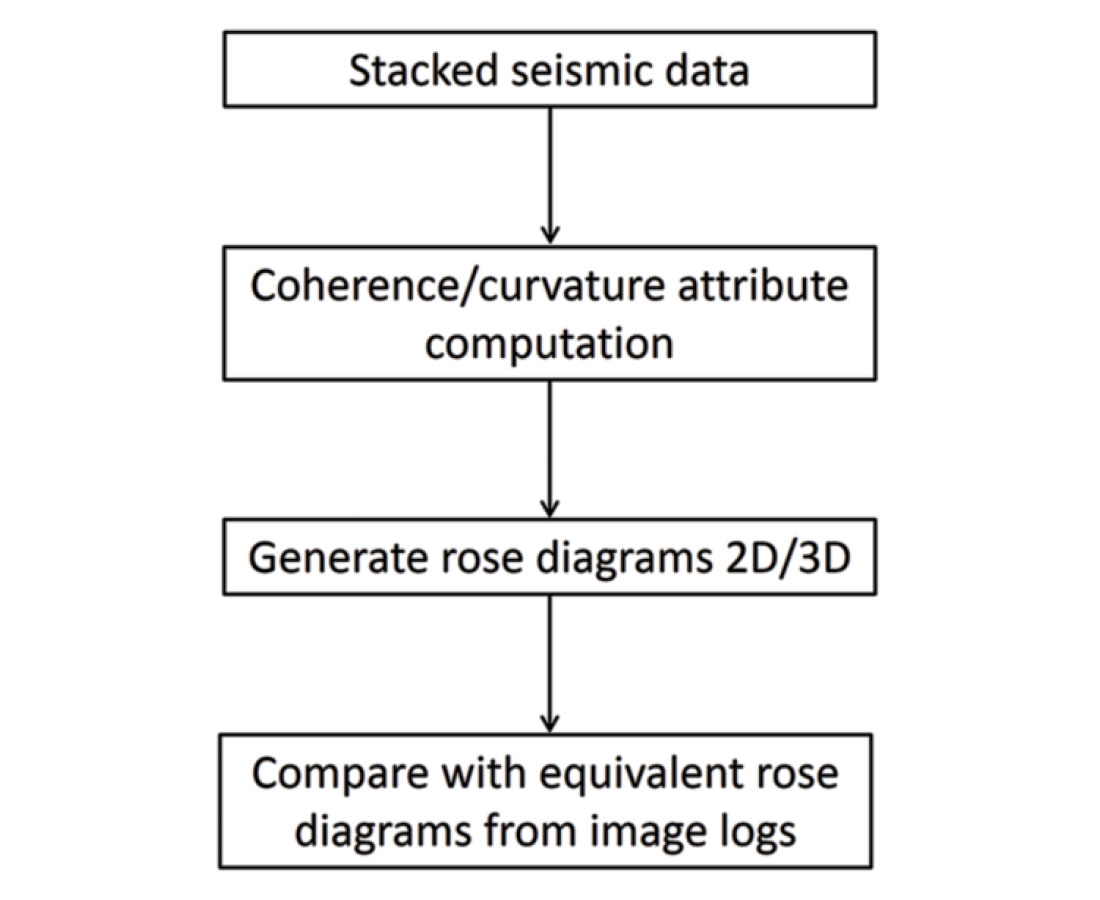
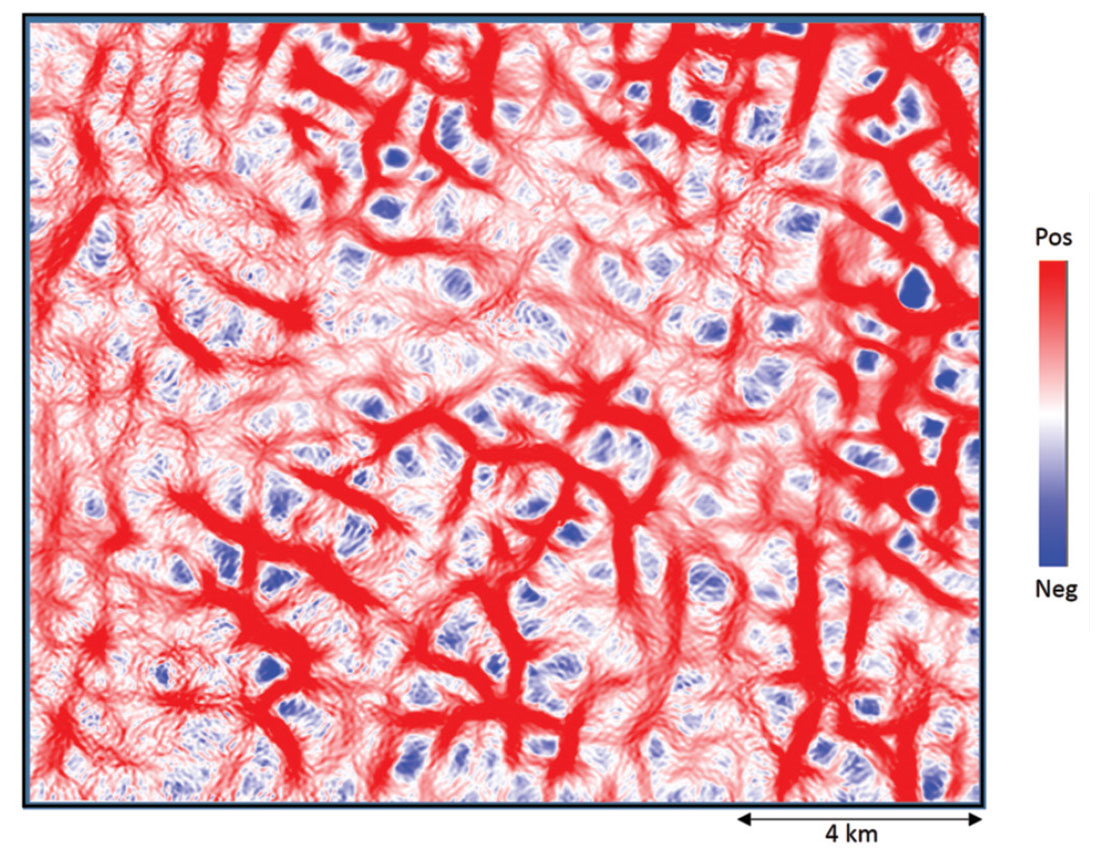
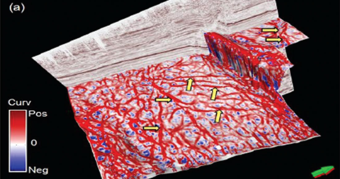
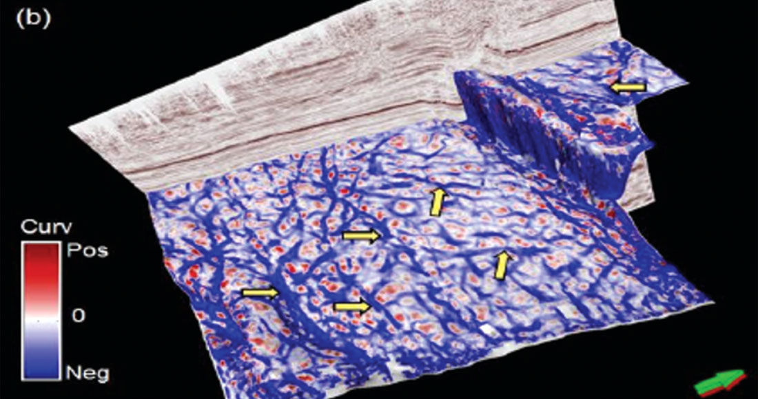
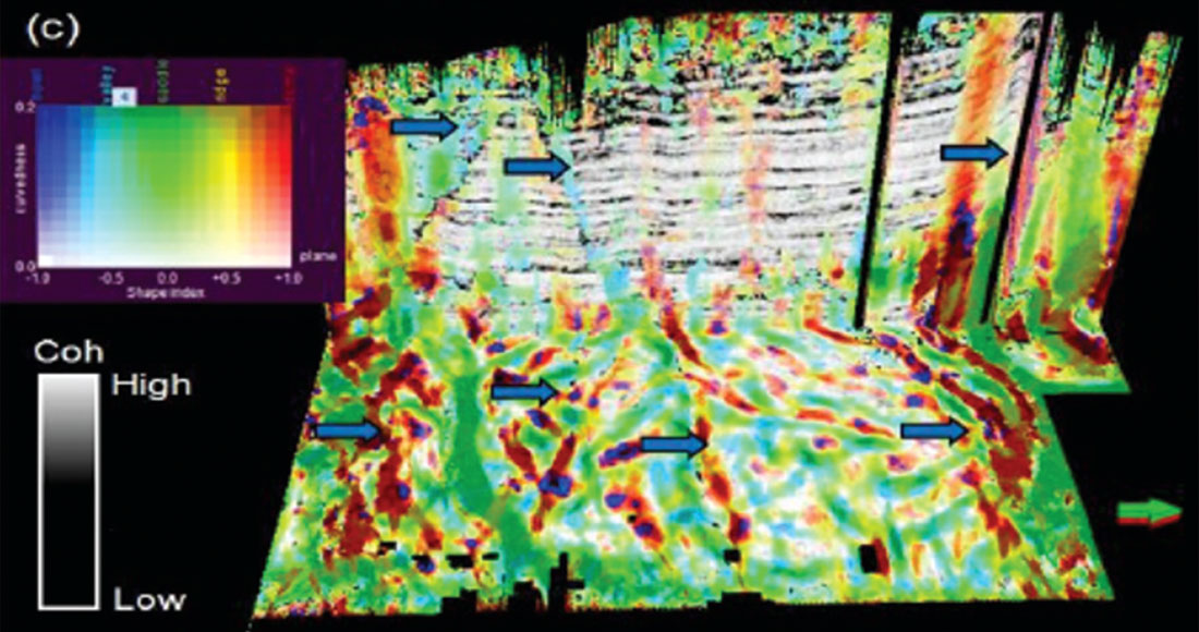
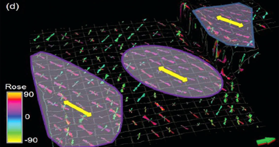
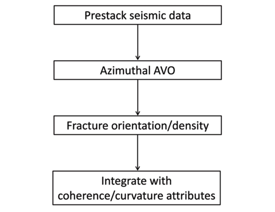
Geometric attributes such as coherence and curvature are commonly used together for mapping fault/fracture lineaments. Using the interpretation for fault/fracture lineaments rose diagrams are generated and calibrated with similar rose diagrams generated from image logs for a more quantitative interpretation. This forms a straight forward workflow for deriving fault/fracture lineament interpretation from post-stack data as shown in Figure 2. Based on such a workflow, in Figure 3 we show a horizon slice through the k₁ most positive curvature attribute which depicts the lineaments depicting the faults and large fractures. Such lineaments interpretation can lead to rose diagrams or 3D rose diagrams may be generated from attributes such as the strike of the maximum curvature and the azimuth of minimum curvature (Chopra et al., 2009). In Figure 4 we show chair diagrams through k₁ most-positive curvature, k₂ most-negative curvature, the structural shape-index modulated by curvedness and co-rendered with coherence, and the 3D rose diagrams from a 3D volume from the Woodford Shale in the Arkoma Basin of Oklahoma. Notice the different orientation of lineaments as indicated with the yellow arrow pockets as compared with the background orientation of NE-SW.

Natural vertical fractures, a consequence of the vertical principal stresses or otherwise, gives rise to horizontal transverse isotropy (HTI). Longitudinally polarized P-waves travel faster parallel to the fractures and slower perpendicular to the fractures, resulting in azimuthal anisotropy. The azimuthal variation in travel time variation is referred to as velocity vs azimuth (VVAz), while the azimuthal variation in reflection coefficients (amplitude) is referred to as amplitude variation with azimuth (AVAz). VVAz requires accurate statics and velocity analysis, does not require amplitude-preserving processing, and provides vertical resolution on the formation by formation (velocity picking) scale. AVAz requires relative amplitude preservation processing. While the output is sample by sample, the resolution is more appropriately approximated by the size of the seismic wavelet. Both VVAz and AVAz yield estimates of the orientation (strike) and intensity of anisotropy. At present, one cannot differentiate between anisotropy due to natural fractures and anisotropy due to lateral variability in horizontal stress (which opens and closes micro fractures). In either case, such information comes in handy when choosing an optimal orientation for horizontal wells (Treadgold et al., 2011; Zhang et al., 2010) mapped anisotropy in survey where the seismic data were acquired after hydraulic fracturing. Such survey may be used in the future to guide infill drilling to exploit by-passed pay or to restimalate a previously stimulated reservoir. These attributes are derived from the conventional 3D seismic surveys using only the vertical prestack P-wave component seismic data and forms a separate workflow as shown in Figure 5.

With multicomponent seismic data, it is possible to add the mode-converted P-S waves (downgoing P-wave converting to an upgoing S-wave) to the data mix. As a P-S wave passes through the vertically aligned fractures, it is split into a fast P-S₁ wave and a slow P-S₂ wave. As with P-waves, the polarization parallel to the fractures is the faster S₁ wave (which travels perpendicular to the fractures). After processing of the recorded data, the time shift Δt in the two types of waves is observed. The simplest product is the difference between S₁ and S₂ time-thickness maps. Such shearwave splitting is attributed to azimuthal anisotropy which can be due to either vertically-aligned fractures or differences between the maximum and minimum horizontal stresses.

Geomechanical properties

The estimation of rock properties from good quality seismic data begins with post-stack impedance inversion, which transforms the seismic amplitudes into impedance values. The impedance data can be correlated with one or more impedance log curves to gain confidence in the performed inversion. Information corresponding to lithology or porosity can be gauged from such an exercise.

Simultaneous AVO inversion uses prestack seismic data to yield P- and, S- impedances and for long offset data, density. Simple arithmetic allows one to compute Poisson’s ratio, V_P / V_S, lambda/mu, lambda-rho, mu-rho, and E-rho. For long offset data, one can compute Young’s modulus (E), lambda, and mu and E-rho. The specific parameterization and lithology “breakout” depends on the rocks, with lambda-rho and mu-rho crossplots being commonly used in carbonates and lithified mudrocks, and P-impedance and Poisson’s ratio being used in less well consolidated Tertiary sands and shales. Much of the engineering literature uses Young’s modulus and Poisson’s ratio, such that E-rho and Poisson’s ratio crossplots might be the method of choice.

The sweet spots in the shale reservoirs are those intervals that exhibit interleaved layers of high brittleness and high TOC, sometimes called “brittle/ductile couplets”. Although high TOC implies a more ductile rock, TOC and chert are often preserved in the same, deeper anoxic part of basin below the upwelling zones where radiolara proliferated. This gives rise to chert-rich brittle rocks that are also TOC-rich. In terms of rock properties, such intervals would be seen to show high Young’s modulus, low Poisson’s ratio, high Mu-rho, low Lambda-rho and high E-rho.

It is not necessary to use a combination of just two attributes at a time for deducing the information on shale reservoirs. It is also possible to use several attributes in conjunction with log curves such as Gamma Ray, porosity and water saturation, and with the use of neural networks or otherwise, map the reservoir zones. A typical seismic survey over a shale reservoir may have ten or more wells with “elastic logs” P-wave sonic, dipole sonic, and density logs. This same survey may encompass hundreds of wells logged only with gamma ray or triple combo logs. By computing a Gamma Ray volume, or a porosity volume, one can correlate the impedance volumes not only to the ten wells with elastic logs, but to the hundreds of wells with gamma ray or triple combo, thus adding more control to the result.

Rickman et al. (2008) showed that brittleness of a rock formation can be estimated from well log curves of Poisson’s ratio and Young’s modulus. This suggests a workflow for estimating brittleness from 3D seismic data, by way of simultaneous prestack inversion that yields Z_P, Z_S, V_P / V_S, Poisson’s ratio, and in some cases meaningful estimates of density. Zones with high Young’s modulus and low Poisson’s ratio are those that would be brittle as well as have better reservoir quality (higher TOC, higher porosity). Such a workflow works well for good quality data and is shown in Figure 6.

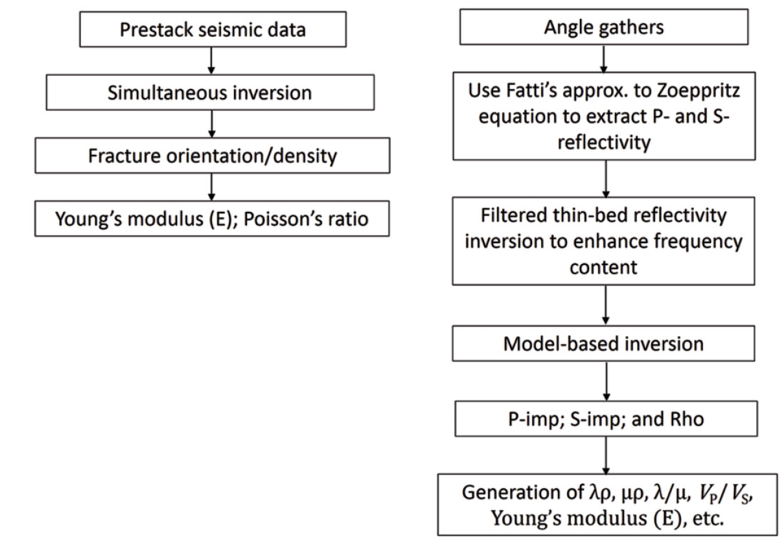
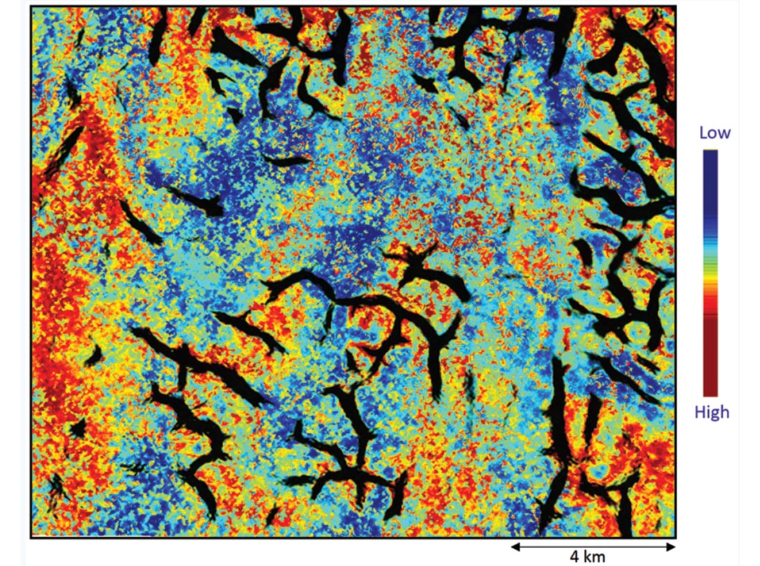
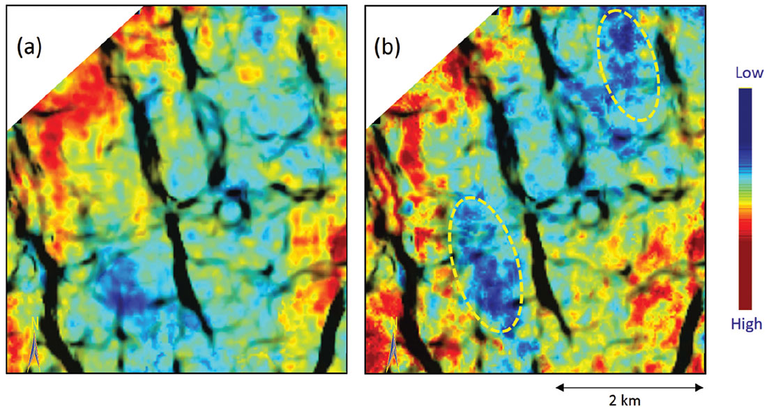
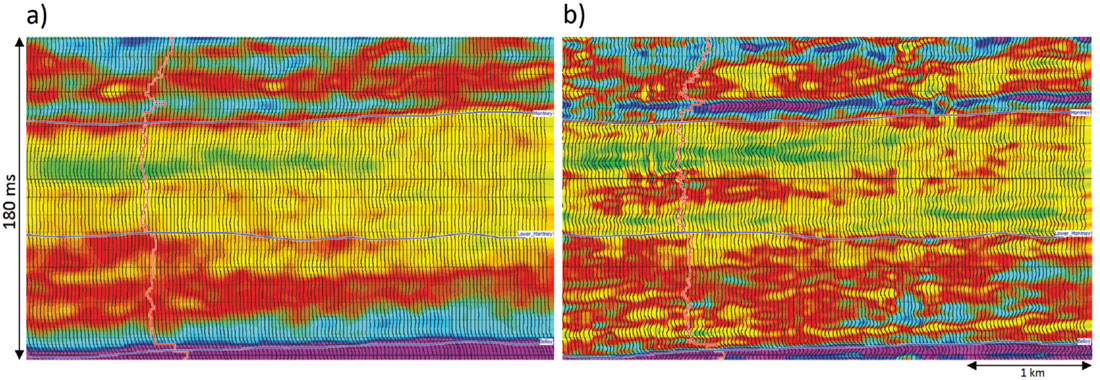
A somewhat different workflow was described by Sharma and Chopra (2013), that results in enhanced resolution of the derived data attributes and hence the desired detail in terms of accurate sweet spot detection. This workflow begins with the angle gathers derived from conditioned offset gathers, from which the P- and S-reflectivity data is derived using Fatti’s approximations to the Zoeppritz equations. A density attribute can also be derived but depends on the quality of the input data as well as the presence of long offsets. Thin-bed reflectivity inversion (Chopra et al., 2006) is now utilized for enhancing the resolution of the P- and S-reflectivity data wherein the effect of the wavelet is removed from the data and the output of the inversion process can be viewed as spectrally broadened seismic data, retrieved in the form of broadband reflectivity data that can be filtered back to any bandwidth. This usually represents useful information for interpretation purposes. Since thin-bed reflectivity removes the seismic wavelet and better estimates a suite of reflection spikes, it better honors the assumptions of “trace integration” relative acoustic impedance. Furthermore, the absence of the seismic wavelet provides a relative acoustic impedance volume that has a higher level of detail. In Figure 7 we show a horizon slice overlay of a k₁ most-positive principal curvature volume seen as black lineaments using transparency with an equivalent slice through the relative acoustic impedance derived from P-reflectivity volume. We notice some patches of low impedance seen bounded by faults and large fracture lineaments. In Figure 8 we show an overlay of the fracture network lineaments using transparency over the relative impedance derived from reflectivity, (a) before, and (b) after frequency enhancement. Notice the different curvature lineaments appear to fall into the appropriate high impedance pockets separating them from low impedance pockets, which may be suggesting cemented fractures.

Similarly, the difference between the Rickman et al. (2008) workflow and the proposed workflow by Sharma and Chopra (2013) is demonstrated in terms of a vertical section comparison as well as a time slice comparison in Figures 9 and 10. The data are taken from the lambda-rho volumes generated by both the workflows. Notice the extra level of detail seen in the proposed workflow.

Next, the output of thin-bed inversion is considered as input for the model based inversion to compute P-impedance, S-impedance and density, which in turn are used to compute other relevant attributes, such as the λρ, μρ and V_P / V_S. These can be used to estimate the pore space properties and other information about the rock skeleton. Young’s modulus can be treated as a brittleness indicator and Poisson’s ratio as TOC indicator.

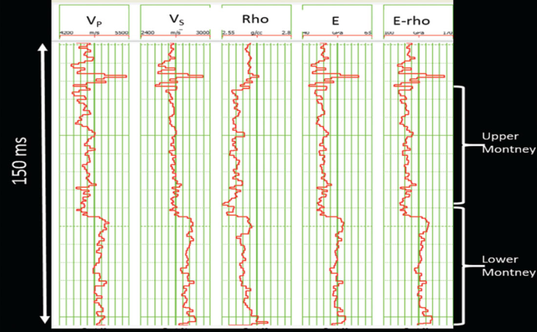
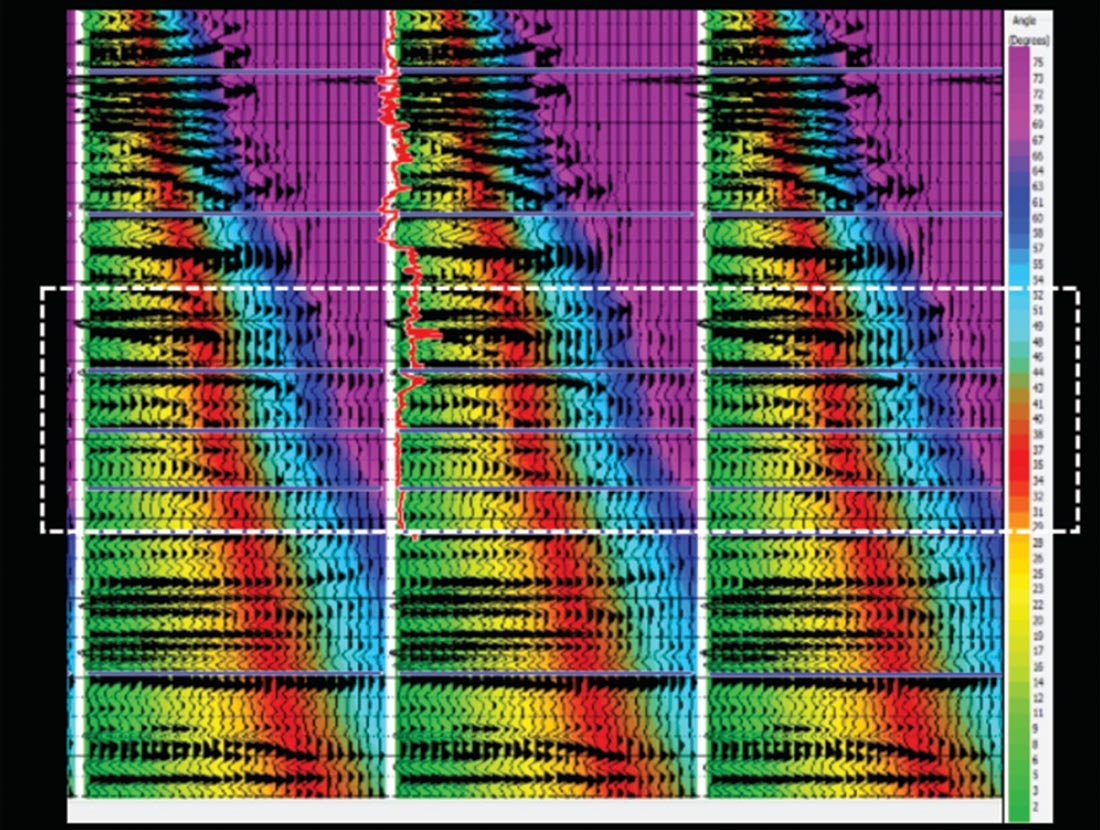
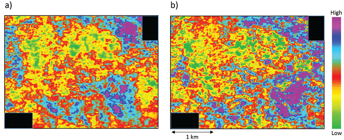
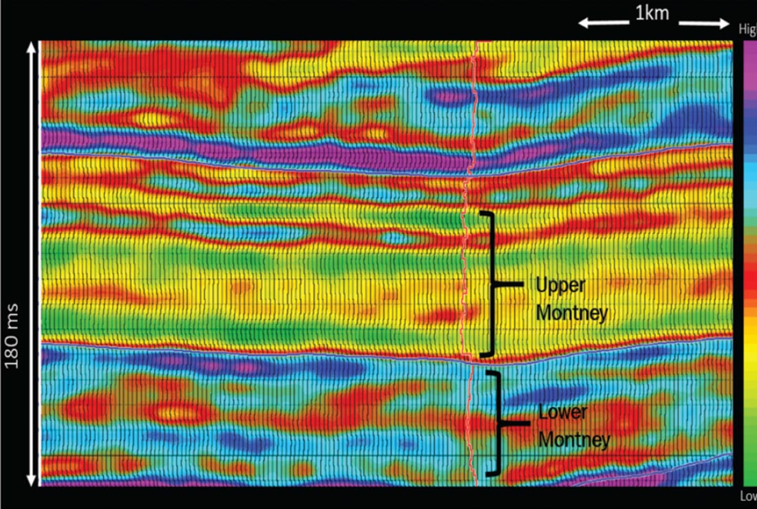
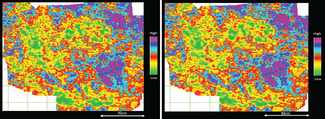
Sharma and Chopra (2013) have demonstrated the generation of E-rho attribute following the integrated workflow shown in Figure 6, and demonstrated that the E-rho curve computed from the log data and compared with the Mu-rho curve shows a higher level of detail. We elaborate on this attribute a little more here. As shown in Figure 11, the computed E-rho curve looks very similar to the E curve. One can cross-correlate these two curves and study their similarity, which in this case showed maximum correlation at zero lag and so high similarity. In an attempt to demonstrate this on real seismic data, we picked up a dataset from the Montney area in NE British Columbia, Canada, which had long offsets, with angles up to 49 degrees. A set of gathers with angles overlaid on them is shown in Figure 12 and the density attribute computed using the 3-term AVO equation is shown in Figure 13. The upper Montney zone exhibits lower values of density as expected, and correlate well with the overlaid density curve. The E-rho attribute was next computed using the integrated workflow shown in Figure 6. A time slice from within the Upper Montney zone averaged over a 10 ms window is shown in Figure 14b. Since both the density and the E-rho datasets were available, it was possible to derive a stand alone Young’s modulus volume. A time slice equivalent to the E-rho slice shown in Figure 14b is shown in Figure 14a. Notice that the two are very similar, confirming the fact that the E and E-rho attributes are very similar.

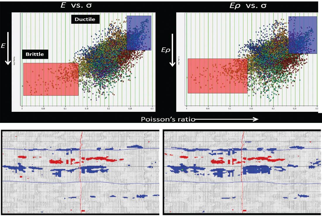
Usually crossplots of E versus Poisson’s ratio are generated to pick out zones of low Poisson’s ratio and high Young’s modulus as these zones would exhibit higher brittleness. In Figure 15 we show crossplots of E and E-rho versus Poisson’s ratio, which look very similar, and even their back projections on the vertical sections look very similar, suggesting that engineering workflows based on E vs. Poisson’s ratio templates can be slightly modified to work on E-rho vs. Poisson’s ratio templates.

Localized stress estimates

The in situ stresses acting on any formation comprise the vertical stress caused by the overburden weight and two horizontal stresses that are a result of the poroelastic deformation of the rocks plus the external tectonic forces. During drilling, a knowledge of the magnitude and direction of in situ stresses is required for design of casing and preventing unwanted open hole strata fracturing in the well. Also, for hydraulic fracture treatment, the in situ stresses have a strong bearing on the fracture azimuth and orientation, fracture width, height, its growth and its conductivity.

These in situ stresses can be estimated from the geomechanical properties determined from seismic data as discussed above. In particular two attributes, namely the differential horizontal stress ratio (Gray et al., 2012; Sena et al., 2011) (DHSR) and closure stress (Goodway et al., 2010) are commonly used for the purpose. DHSR is the ratio between the maximum and minimum horizontal stresses to the maximum horizontal stress. Zones with low DHSR values, could have fractures formed in a random manner and so creating a fracture swarm. Thus low DHSR values are favorable. Closure stress is the minimum pressure required to hold open a fracture once it is created. Optimal producing zones would exhibit high Young’s modulus and low DHSR or closure stress values. The derivation of stress estimates from some of the attributes discussed above would be discussed at another time.

Conclusions

Geophysical methods can help in characterizing the shale gas resource plays. However, the methodology adopted is in general different from methodologies applied to conventional reservoirs. Specifically, because of the significantly greater well control, shale resource plays are much more amenable to a more quantitative interpretation. While the workflows can in general be applied to most shale plays, the characterization of each shale reservoir may require particular types of tools and formation specific or even survey specific templates. While we have discussed a number of different workflows for characterization of shale gas reservoirs, the choice of such methods will continue to evolve to meet the growing challenges and expectations.

Acknowledgements

We thank Arcis Seismic Solutions, TGS for encouraging this work and for permission to present these results.